UDK 624.014.046;519.853
Linearna in nelinearna ravnovesna enačba v računalniško podprtem konstruiranju
A Linear and a Nonlinear Equilibrium Equation in CAD of Structures
MAKS OBLAK - MARKO KEGL - BRANKO BUTINAR
V prispevku obravnavamo vpeljavo nelinearne ravnovesne enačbe v postopek optimalnega projektiranja konstrukcij, pri katerem se je doslej v glavnem uporabljala linearna enačba. Če v nelinearni enačbi upoštevamo končne pomike in zasuke, naletimo pri tem na težave v zvezi z nestabilno ravnovesno krivuljo konstrukcije. Standardno optimalno projektiranje je zaradi tega praktično neuporabno. Nov prijem, ki je predstavljen v prispevku, temelji na modificiranem problemu optimalnega projektiranja in spremenljivi ravni obremenitve. Ponazorjen je na dveh zgledih, na katerih je tudi narejena primerjava med uporabo linearne in nelinearne enačbe.
The paper discusses the introduction of a nonlinear equilibrium equation into the optimal design of structures where a linear equation has been mostly used to date. If kinematic nonlinear effects enter the equilibrium equation, difficulties can arise owing to an unstable equilibrium path of the structure. Because of that, the classic approach to optimal design becomes practically unusable. The new approach presented in this paper is based on a modified problem of optimal design and a variable load level. It is illustrated with two examples where the use of linear and nonlinear equilibrium equations is also compared.
0. UVOD
Optimalno izbiranje konstrukcijskih para metrov pomeni dandanes že sestavni del računal niško podprtega projektiranja (CAD) konstrukcij. Gre za avtomatično določanje optimalnih vrednosti nekaterih konstrukcijskih parametrov, ki do te faze projektiranja še niso izbrane, na primer di menzije in oblike robov posameznih delov kon strukcije, karakteristike geometrijske oblike pre rezov, vrste materiala, smeri podprtja konstrukci je in podobno.
V računalniško podprtem projektiranju kons trukcij predpostavljamo, da imamo na voljo ravno vesno enačbo, iz katere lahko pri danih obreme nitvah izračunamo odziv, ki dovolj dobro ustreza dejanskemu. Rutinsko nastajanje takšne enačbe omogoča za večino konstrukcij metoda končnih elementov (MKE). Če so izpolnjene zahteve:
a) pomiki vozlišč so zanemarljivo majhni, b) robni pogoji se med obremenjevanjem ne
spreminjajo,
c) material je linearno elastičen,
je ravnovesna enačba linearna. V nasprotnem pri meru je linearna enačba neustrezna 111 in upora biti moramo nelinearno. Glede na izpolnjevanje pogojev a) do c) delimo vzroke za nelinearnost enačbe konstrukcije v kinematične in materialne. Prvi so posledica neizpolnjenih pogojev a) ali b), drugi pa neizpolnjenega pogoja c).
0. INTRODUCTION
Optimal selection of design parameters - op timal design - is today an integral part of compu ter aided design (CAD) of structures. It involves the automatic determination of optimal values of some design parameters which are still undeter mined in the current stage of design, for example, dimensions and shapes of structural parts, geo metric properties of cross-sections, material pro perties, directions of supports and so on.
In CAD of structures, we assume that we have an equilibrium equation at our disposal from which we can calculate the structural response for given loads with satisfactory accuracy. For most structures, this equation can be successfully generated using the finite element method (FEM). If the following requirements are fulfilled:
a) nodal displacements are negligibly small, b) boundary conditions do not change during
loading.
c) the material is linear elastic,
Razvoj optimalnega projektiranja v okviru CAD je v zadnjih dvajsetih letih temeljil na upo rabi linearne ravnovesne enačbe, kar je tudi raz vidno iz ponudbe komercialno dosegljivih raču nalniških programov. Uporaba nelinearne enačbe se v inženirski praksi še ni uveljavila predvsem zaradi težav, ki preprečujejo, da bi v že razvitem postopku optimalnega projektiranja linearno enačbo konstrukcije zamenjali z nelinearno. Te se lahko pojavijo pri neizpolnjevanju pogoja a) in se nana šajo na stabilnostne lastnosti mehanskega sistema. Nekaj poskusov odpravljanja teh težav smo v zadnjih letih sicer lahko opazili 121, vendar so bili rezultati precej skromni.
V Laboratoriju za optimiranje mehanskih sistemov na Tehniški fakulteti v Mariboru smo razvili nov način optimalnega projektiranja sta tično obremenjenih konstrukcij, ki omogoča učinkovito uporabo nelinearne ravnovesne enačbe tudi pri upoštevanju velikih pomikov. Na tej pod lagi smo razvili programsko opremo za optimalno projektiranje paličnih konstrukcij in na zgledih potrdili uporabnost novega načina.
1. RAVNOVESNA ENAČBA KONSTRUKCIJE IN RAVNOVESNA KRIVULJA
Če predpostavimo uporabo metode končnih elementov in se omejimo na statično obremenjene konstrukcije brez učinkov lezenja, lahko ravno vesno enačbo konstrukcije v splošni obliki zapi šemo 111:
0(1
n n
kjer je Q( u) e M , u e IR pa je vektor vozliščnih pomikov in zasukov.
Enačbo (1) imenujemo linearna ravnovesna enačba, če je funkcija Q linearna glede na spre menljivko u. V tem primeru (1) zapišemo v obi čajni obliki:
K u
kjer sta /ftogostna matrika konstrukcije, R n pa vektor zunanjih vozliščnih obremenitev. To- gostna matrika K in vektor obremenitev R sta konstantna in neodvisna od pomikov u. Reševanje ravnovesne enačbe je z matematičnega vidika ne problematično, saj je treba rešiti sistem linearnih enačb, čigar matrika je simetrična, pasovna in vedno dobro pogojena.
Kadar je funkcija Q nelinearna glede na spre menljivko u, imamo nelinearno ravnovesno enačbo. V tem primeru togostna matrika konstrukcije ali vektor zunanjih obremenitev nista konstantna in sta odvisna od pomikov u. Reševanje nelinearne enačbe nadomestimo 131 z reševanjem zaporedja enačb:
Development in the field of optimum design in CAD was based on the use of a linear equilibrium equation, which is also evident from the supply of commercially available computer programs. The use of a nonlinear equation could not be establi shed in practical engineering tasks owing to diffi culties in replacing a linear equation with a non linear one in a well-formed procedure of optimal design. These difficulties, which concern structu ral stability properties, can appear if condition a) is not fulfilled. Some attempts to solve these dif ficulties have already been made 121, but the re sults have been rather modest.
In the Laboratory for optimum design of mechanical systems at the Technical Faculty in Maribor, a new approach to optimum design of statically loaded structures has been developed, which enables effective use of a nonlinear equi librium equation accounting also for large displa cements. On this basis, software for the optimum design of truss structures has been developed and its usefulness has been confirmed on several examples.
1. THE EQUILIBRIUM EQUATION OF THE STRUCTURE AND THE EQUILIBRIUM PATH
If we suppose the use of the finite element method and if we restrict ourselves to statically loaded structures, we can write the equilibrium equation of the structure in a general form 111 as:
= 0 (1),
where Q( u) e R n, u e R " represents the vector of nodal displacements and rotations.
Equation (1) is termed to be a linear equili brium equation, if the function Q is linear with respect to the variable u. In this case (1) is commonly written as:
R
where K is the structural stiffness matrix and R e [R 71 is the vector of external nodal loads. From the mathematical point of view, solving the linear equilibrium equation causes no difficulties since it is necessary to solve a linear system of equations where the coefficient matrix is sym metric, banded and always well-conditioned.
Q{u,t) = O, t = t 0, t i . . . , t j, ć0 = 0 , f j = l (2) ,
kjer t pomeni neodvisno spremenljivko, ki ima pri statičnih problemih brez učinkov lezenja vlogo označevanja intenzivnosti obremenitve (inkre- mentni postopek). Vsaka enačba iz zaporedja (2) je sicer nelinearna, vendar lahko njeno rešitev t u iz računamo preprosteje, če je obremenitveni inkre- ment ( - tj ) majhen. Postopek reševanja je iteracijski in ga lahko z označbami r = £J+, in s = tj zapišemo 111 :
r ( o ) s
II = II ;
r ( i +1 ) r ( i )
II = II +
kjer je N0 množica pozitivnih celih števil. Pri tem izračunamo Au(i+1) iz enačbe:
where t represents an independent variable, which in static analysis without creep effects merely denotes the imposed load level (incremen tal procedure). Each equation from the sequence (2) is still nonlinear, but its solution tl can be more easily obtained if the load increment ( tj +1 - tj ) is small. The solution procedure is iterative and can be written 111 with the symbols r = tj +i and s = tj as:
where is a set of non-negative integer numbers. The increment A u 1 + is calculated from:
v o)
kjer je qK tangentna togostna matrika 111 kon strukcije pri ravni obremenitve q t Itj, £J + 11, ki je odvisen od izbrane tehnike reševanja, J5* e 1R pa je vektor notranjih sil, izračunan na podlagi napetostne porazdelitve, pri nivoju obre menitve r. Reševanje (3) zahteva invertiranje tangentne togostne matrike. Če so zunanje obre menitve neodvisne od pomikov, je ta matrika sicer še simetrična in pasovna, ni pa več vedno dobro pogojena.
Z vpeljavo neodvisne spremenljivke t lahko definiramo množico:
= >
where qK is the structural tangent stiffness matrix 111 at load level q ? 1 £.-, £J + 11, q de pend on the chosen solution technique, and ' F e IRn is a vector of internal forces (calculated from the stress distribtion) at load level r. To solve (3) it is necessary to invert the tangent stiffness matrix. If the external loads are displa cement independent, this matrix is still symmet ric and banded, but it is no longer always well- -conditioned.
By introducing the independent variable t one can define the set:
t/= { V 0(o, t) = 0, Os f s 1},
ki jo imenujemo ravnovesna krivulja konstrukcije. Ravnovesna krivulja je v točki t u stabilna 141, če je d e tC /f) > O, oziroma nestabilna, če je det(t Ä') < 0. Točko, v kateri ni ravnovesna kri vulja niti stabilna niti nestabilna, imenujemo kritično točko. V kritični točki, ki jo bomo ozna čili z cu, je izpolnjen pogoj:
which is termed the equilibrium path of the structure. An equilibrium path is said to be stable 141 at the point *11 if det Č /f) > 0 , and unstable if
d e t^ /f) < 0 respectively. The point at which the equilibrium path is neither stable nor unstable is called a critical or stability point. At the critical point, which will be denoted by cu, the following condition is fulfilled:
det (CK) = 0,
kjer je CK tangentna togostna matrika pri nivoju tc . Obremenitveni nivo tc, ki ustreza točki cu imenujemo kritični nivo obremenitve.
V grobem delimo kritične točke na mejne in bifurkacijske 141. Pri povečanju obremenitve prek tc postane pri mejnih točkah ravnovesna krivulja nestabilna, medtem ko se pri bifurkacijskih razce pi na primarno in sekundarne veje. Natančnejša razdelitev kritičnih točk zahteva precej računske ga dela in je podrobno opisana v 141.
where CK is the tangent stiffness matrix at load level tc . The load level tc corresponding to the point Ln is called the critical load level.
2. VPELJAVA NELINEARNE RAVNOVESNE ENAČBE V OPTIMALNO PROJEKTIRANJE
KONSTRUKCIJ
Namen optimalnega projektiranja je določitev najboljših vrednosti nekaterih konstrukcijskih pa rametrov, ki so do te stopnje projektiranja še nedoločeni. Označimo te parametre z a « IRm . Razumljivo je, da vrednost a vpliva na odziv konstrukcije pri dani obremenitvi, kar pomeni, da se vektor a pojavlja v ravnovesni enačbi kon strukcije (1).
Ker pri optimalnem projektiranju konstruk cijske parametre obravnavamo kot spremenljivke, moramo torej ravnovesno enačbo v tem primeru zapisati nekoliko drugače:
2. INTRODUCTION OF A NONLINEAR EQUILIBRIUM EQUATION INTO THE OPTIMUM DESIGN OF STRUCTURES
The purpose of optimum design is to evaluate the optimum values of some design parameters which are still undetermined in the current stage of design. Let us denote these parameters with a e [Rm. It is clear that the value of a influences the response of the structure at given loads, which means that a is included in the equilibrium equation (1) of the structure.
Since in optimum design the design para meters are treated as design variables, we have to write the equilibrium equation in a slightly different way:
(4), C (u,a) = 0
kjer je Gi u, a) e IRn . Ravnovesno enačbo zapisa no v obliki (4) imenujemo tudi enačba stanja.
Optimalne vrednosti konstrukcijskih pa rametrov ustrezajo zahtevam projektanta, ki jih mora v matematični obliki izraziti z uporabo namenske funkcije in omejitvenih pogojev. Tako lahko problem optimalnega projektiranja zapi šemo v obliki problema matematičnega progra miranja:
min
ob upoštevanju pogojev:
gj (u,a) š
where G l u , a) e R n An equilibrium equation of the form (4) is also termed a state equation.
Optimaum values of design parameters corre spond to the requirements of the designer which has to be expressed in a mathematical form by an objective function and constraints. In this manner, the problem of optimum design can be written in - the form of a problem of mathematical pro gramming:
f l a )
(5), subject to constraints
(6)
in enačbe stanja:
G(u
kjer so f — namenska funkcija, gj — skalama funk cija (pomik vozlišča, napetost itn.), katere vred nost želimo omejiti, g j ~ pa je njena največja do pustna vrednost. V problemu (5) —(7) se pojavlja poleg namenske funkcije v (5) in omejitvenih po gojev (6) tudi enačba stanja (7). Razlog je v tem, da se v (6) odvisna spremenljivka u ne da izraziti eksplicitno v odvisnosti od spremenljivke a. Njuna povezava je zato implicitno podana s (7).
Problem (5)—(7) je praktično vedno nelinea ren. Rešitev a * zato običajno izračunamo kot li mito zaporedja ( a (l)), ki ga naredimo takole:
— a (o) izberemo;
— a (1 + 1) določimo kot rešitev problema P (1), ki je definiran na podlagi problema (5) —(7) ter točke a Cl) in, i € |\l0.
and the state equation
i) = 0 (7)’
where f — is the objective function, gj — is a scalar function (nodal displacement, effective stress, etc.), whose value has to be restricted and g, is its limiting value. Besides of the objec tive function (5) in the constraints (6), the pro blem (5)—(7) also includes the state equation (7). The reason is that in (6) the dependent variable u cannot be expressed explicitly in terms of the independent variable a Therefore, the relationship between u and a is implicitly given by (7).
The problem (5)—(7) is almost always non linear. Its solution a is therefore usually calcu lated as a limit of the sequence ( a (1)), which is generated in the following way
— a (o) has to be chosen;
Pri tem je lahko izbira a (o) precej poljubna, problem matematičnega programiranja P (l) pa najpogosteje definiramo, kot aproksimacijo pro blema (5)—(7) v točki a (i) . Nastajanje problema - P (1) terja izračun mnogih vrednosti, vendar je najpomembnejši in računsko najzahtevnejši izra čun odziva u in odvoda du/ da v to č k ia (i) [51. Oba izračuna opravimo na temelju enačbe stanja (7).
Pri uporabi linearne ravnovesne enačbe je funkcija G v (7) linearna glede na u. Omenili smo že, da lahko takšno enačbo uporabimo le ob nekaterih predpostavkah, ki sicer niso preprosto določljive. K temu je treba dodati, da je veljavnost linearne enačbe odvisna tudi od vrednosti kon strukcijskih spremenljivk. Ker se pri optimalnem projektiranju te vrednosti iz iteracije v iteracijo spreminjajo, se lahko znajdemo v še posebej te žavnem položaju, tako da postane vpeljava ne linearne ravnovesne enačbe nujno potrebna.
Preprosto obravnavanje problematike bi nas lahko pripeljalo do sklepa, da terja vpeljava ne linearne ravnovesne enačbe le uporabo nelinearne funkcije G glede na spremenljivko u. To je celo res pri upoštevanju nekaterih nelinearnosti, kakor je na primer materialna. Toda ob pozornejšem pregledu lahko hitro ugotovimo, da bi tako na leteli na nepremagljive ovire, če ne bi upoštevali vseh mehanskih in matematičnih vidikov pro blema.
Pri upoštevanju kinematičnih nelinearnosti obstaja namreč možnost, da bo v poljubni iteraciji (v točki a (1)) ravnovesna krivulja konstrukcije odsekoma nestabilna. Takšne razmere so običajno z inženirskega vidika nesprejemljive, saj to po meni, da odziva konstrukcije ni mogoče popolnoma napovedati. Pri povečanju obremenitve čez mejno točko pride namreč do »preskoka« konstrukcije v močno deformirano stanje, medtem ko lahko pri bifurkacijski točki odziv ob povečanju obre menitve ustreza različnim vejam ravnovesne krivulje. V obeh primerih lahko pride do porušitve konstrukcije.
Zaradi tega moramo problemu (5) —(7) pri upoštevanju kinematičnih nelinearnosti obvezno dodati stabilnostni pogoj:
Čeprav bi lahko sklepali, da bodo s tem teo retične težave odpravljene, so v praksi stvari precej drugačne. Pogoj (8) bo namreč zanesljivo izpolnjen le v optimalni točki a*, medtem ko za poljubno točko a (1) tega ne moremo pričakovati. Torej se lahko zgodi, da bo v poljubni iteraciji tangentna togostna matrika na nekaterih nivojih obremenitve slabo pogojena ali celo singularna.
The choice of a (o)can be quite arbitrary while the problem of mathematical programming P (1)is mostly defined as an approximation of the problem (5)—(7) at the point a (1). Generation of the pro blem P (i) requires the evaluation of many quanti ties. However, the most important and most diffi cult is the calculation of the response uand the de rivative du/daat the point a (1) [51. Both calcula tions are performed by using the state equation (7).
If a linear equilibrium equation is used, then the function Gin (7) is linear with respect to the variable u As it has already been mentioned, such an equation can only be used on some assumptions which are not simple to predict. In addition, the validity of the linear equation depends also on the values of design variables. Since in optimum design these values change from iteration to ite ration, we are confronted with a quite difficult situation, making the introduction of a nonlinear equation necessary.
A naive treatment of this subject could yield the conclusion that the introduction of a nonlinear equilibrium equation only requires the use of a nonlinear function G w ith respect to the variable if. This is even true when some of the nonlinear effects are considered, for example, the material nonlinearity. However, it can be seen that consi dering kinematic nonlinearities in this case, we would soon meet some insuperable problems if all of the mechanical and mathematical aspects of the problem were not considered.
In other words, in considering kinematic nonlinearities, there exists the possibility that in an arbitrary iteration (at the point a (i)) the equi librium path of the structure is partially unstable. From an engineering point of view, such conditi ons are usually unacceptable since in this case the structural response is not completely predictable. Increasing the load level over the critical value leads to snap-through at the limit points while at the bifurcation points, the response may corres pond to different branches of the equilibrium path. In both cases, the structure may collapse.
Because of that, when kinematic nonlinea rities are considered, we have to add to the problem (5)—(7) the stability constraint:
(8) ,
Ker terja nastajanje problema P (lj reševanje linearnih sistemov enačb, katerih sistemska matrika je tangentna togostna matrika, lahko pričakujemo numerične težave. V praksi velja, da je dejansko stanje še nekoliko slabše, saj se pojavijo tudi težave v zvezi s konvergenco za- porednja ( a (1)) in veliko računsko neučinkovi tostjo takega načina.
Nov način, ki smo ga razvili v Laboratoriju za optimiranje mehanskih sistemov, zelo učinkovito odpravlja vse opisane težave. Bistvo novega načina je v tem, da P (i) določimo kot aproksimacijo problema:
P (1)requires the solution of a system oflinear equa tions with the tangent stiffness matrix as the coefficient matrix, one can expect numerical diffi culties. Actually, in practical tasks, the conditions are even worse due to difficulties concerning the convergence of the sequence ( a ( n ) and the extreme inefficiency of such approach.
The new approach, which has been developed in the laboratory for optimum design of mechanical systems, avoids all the above mentioned difficul ties in a very effective way. The essence of the new approach is that is determined as an ap proximation of the problem:
i
min /Ta) (9),
ob upoštevanju pogojev: subject to constraints:
gj (iI,a) É (p(1)g ), j = 1, ..., k
w (ti, a) ž 1,
in enačbe stanja: anc^ the state equation:
G(u,a, p (i)) = 0
(10)
(11)
(12) , v točki a (i), kjer je w(u, a) ocena kritične
obremenitvene ravni, tako da je w (cu,a) = = /c (a), s p li) pa smo označili fiksno raven obremenitve, ki jo določimo med analizo odziva (reševanje enačb (2)) s preverjanjem naslednjih pogojev:
1)
at the point a (i), where w( u ,a) is an estimation of the critical load level, so that w (cu,a) = = /c (a), and p (1) is a fixed load level which is determined during response analysis (while sol ving equations (2)) by checking the following conditions:
t = 1; (13)
2) / = Z c (a(1)); (14)
3) max {gj (*11, a (1)) / (t gj) - 1 ; j = 1, ..., A' } ž 1 - t (15).
Če je katerikoli izmed pogojev (13)—(15) iz polnjen, vrednost parametra t priredimo para metru p (1) in analizo odziva končamo.
Bistveni razliki med problemoma (5)—(7) in (9)—(15) sta dodana ocena stabilnostnega pogoja in prilagodljiva raven obremenitve, za katero zaradi ( 13)—( 15) veljap(i) é min {l, /c ( a t n )}. Dodan ocenjen stabilnostni pogoj zagotavlja pra vilnost rešitve a * prilagodljiva raven obre menitve pa učinkovit in numerično zanesljiv numerični postopek optimalnega projektiranja. Pokažemo lahko (6), da zaporednje ravni p (i\ ki ustreza zaporedju a (i), konvergira k 1. Zaradi tega sklepamo, da lahko problem (5)—(7) vedno nadomestimo z (9)—(15).
If any of the conditions (13)—(15) is fulfilled, then the value of p (1) is set to be equal to the value of / and the response analysis is terminated.
Učinkovita numerična uporaba novega načina zahteva seveda precej več ko zgolj opisani posto pek, vendar bomo, zaradi preglednosti, podrobnosti v tem prispevku izpustili. Omenimo le, da je novi način v celoti opisan v 161 in 171.
3. ZGLEDI
Slabosti uporabe linearne ravnovesne enačbe si oglejmo na dveh reprezentativnih zgledih. V obeh primerih gre za palične konstrukcije, pri ka terih so že določene koordinate vozlišč, topologija, gradivo, podprtje in obremenitve. Nedoločeni so le še prerezi posameznih elementov. Te bi radi izbrali tako, da bo prostornina porabljene snovi minimal na. Pri tem napetosti v posameznih elementih ne smejo preseči predpisane vrednosti. Izbrani mate rial lahko v pričakovanem območju obremenjeva nja (dopustne napetosti) obravnavamo kot linearno elastičen.
Izmed zahtev a) do c), ki upravičujejo uporabo linearne enačbe, sta izpolnjena pogoja b) in c). Glede pogoja a) za zdaj še ne moremo reči ničesar, saj je odvisen od deformacij konstrukcije pri polni obremenitvi. Na dveh računskih zgledih bomo pokazali, da brez uporabe nelinearne enačbe prav zaprav ne vemo, ali je pogoj a) izpolnjen ali ne. Torej je uporaba nelinearne enačbe mnogokrat - nujno potrebna, če se želimo izogniti neprijetnim posledicam.
Za zgled smo uporabili dve izmed standardnih konstrukcij, ki se pojavljajo v specializirani lite raturi v zvezi z razvojem postopkov optimalnega projektiranja. Zaradi tega bomo tudi uporabili iz virne številčne podatke. Za njihov preračun v sistem SI je te številčne vrednosti treba pomno žiti s konstantami in enotami, ki so navedene v
151. Oba zgleda sta rešena z aproksimacijsko me todo matematičnega programiranja (aproksimacija s tremi parametri) I8I.
Zaradi jasnosti prikaza rezultatov se še do govorimo, da bomo uporabljali naslednji označbi:
OPT_L — optimalna konstrukcija, dobljena z upo rabo linearne enačbe;
OPT_N — optimalna konstrukcija, dobljena z upo rabo nelinearne enačbe.
Označbi OPT_L in OPT_N pomenita dve varianti iste konstrukcije. Ustreznost ali ne ustreznost variante OPT_L bomo preverili z analizo odziva konstrukcije z uporabo nelinearne ravnovesne enačbe, ki natančneje opisuje dejanski odziv.
An effective numerical implementation of the new approach requires of course some further discussion, but for the sake of brevity in this paper the details will be omitted. It should just be noted that a detailed description of the new approach can be found in 16] and 171.
3. EXAMPLES
The drawback of using a linear equilibrium equation will be illustrated with two examples. Both cases involve truss structures with known nodal coordinates, topology, material properties, as well as support and loading conditions. Still unde termined are the cross-sections of individual ele ments. These should be chosen in such a way that the volume of the material used will be minimum. At the same time, the stresses in individual mem bers may not exceed the prescribed values. The chosen material can be treated as linear elastic in the expected range of loading (allowable stresses).
Among the conditions a) to c) which justify the use of a linear equation, conditions b) and c) are fulfilled. However, nothing can be concluded yet about condition a) since it depends on the amount of deformation at full loading. On two numerical examples, it will be shown that without using a nonlinear equation we actually do not know whet her condition a) is fulfilled or not. The use of a nonlinear equation is thus necessary if we wish to avoid unpleasant consequences.
In the examples, we used two standard structures which frequently appear in the specia lized literature in connection with the develop ment of optimum design procedures.. We will therefore also use the original numeric data. To express this data in the SI system these numbers should be multiplied by the constants and units given in 151. Both examples have been solved by using an approximation method of mathematical programming (three-parameters controlled approximation) I8I.
For the sake of clarity, we will use the following notations:
OPT_L— the optimum structure obtained with the use of a linear equation
OPT_N — the optimum structure obtained with the the use of a nonlinear equation.
3.1 Paličje z desetim i elem enti 3.1 The 10-bar tru ss
Konstrukcija je prikazana na sliki 1, kjer so tudi razvidne koordinate vozlišč, topologija in pod prtje. Izbran material ima elastični modul E = = 30000 ksi, največ ja dopustna napetost pa je Iödopl = 20 ksi. Zunanja obremenitev/? = -10 kips deluje v navpični smeri v vozliščih 2 in 4. Prerez posameznega elementa ne sme biti manjši od ® m l n — •
The stucture is shown in figure 1, where the coordinates, the topology and the support condit ions can also be seen. The chosen material has an elastic modulus E = 30000 ksi and the greatest allowable stress is |ddop| = 20ksi. The external load R = -10 kips acts in a vertical direction at nodes 2 and 4. The cross-section of an individual element may not be smaller than a min = 0.1 in2.
3 6 0 3 6 0
Sl. 1. Paličje z desetimi elementi. Fig. 1. The 10-bar truss. Paličje smo optimirali z uporabo linearne in
nelinearne ravnovesne enačbe. Rezultati optimi ranja so podani v preglednicah 1 in 2.
The truss has been optimized by using the linear as well as the nonlinear equilibrium equa tion. The results of the optimization are listed in tables 1 and 2.
Preglednica 1: Optimalna prostornina. Table 1: Optimum volume
OPT_L OPT_L
2071,8 2071,4
Preglednica 2: Optimalni prerezi Table 2: Optimum cross-sections
OPT_L OPT_N
a, 1,0621 1,0600
a2 0,4379 0,4370
a3 0,1000 0,1000
a4 0,1000 0,1000
as 0,9379 0,9382
a6 0,1000 0,1000
a7 0,6192 0,6202
3q 0,7950 0,7944
a9 0,1000 0,1000
a io 0,6192 0,6199
Iz preglednic 1 in 2 vidimo, da sta varianti From tables 1 and 2, it can be seen that OPT_L in OPT_N praktično identični. To pomeni, options OPT_L and OPT_N are practically iden-da je v tem primeru linearna enačba dovolj dobra. tical. This means that in this case, the linear Potrditev te ugotovitve lahko najdemo tudi v equation is good enough. This can be confirmed preglednicah 3 in 4, kjer so podani vozliščni po- by inspecting tables 3 and 4, where nodal displa-miki in napetosti obeh variant, izračunani
rabo nelinearne enačbe.
Preglednica 3: Odziv konstrukcije
(pomiki — nelinearna enačba)
Table 3: Sructural response
(displacements — nonlinear equation)
OPT_N OPT_L
«v U y ux U y
v, 0,387 -1,771 0,387 -1,771
v 2 -0,483 -1,919 -0,482 -1,919
v3 0,239 -0,720 0,239 -0,720
v4 -0,241 -0,720 -0,240 -0,720
Preglednica 4: Odziv konstrukcije Table 4: Structural response
(napetosti — nelinearna enačba) (stresses — nonlinear equation)
OPT_N OPT_L
-19,994 - 19,966
-19,991 -19,951
*3 12,424 12,437
12,416 12,429
19,998 19,997
0,044 - 0,018
-19,995 -20,009
19,997 19,996
*3 -17,561 -17,578
Ö,0 19,991 20,011
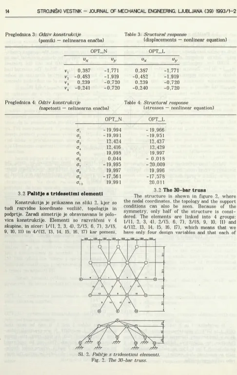
3.2 Pallčje s tridesetim i elem enti
Konstrukcija je prikazana na sliki 2, kjer so tudi razvidne koordinate vozlišč, topologija in podprtje. Zaradi simetrije je obravnavana le polo vica konstrukcije. Elementi so razvrščeni v 4 skupine, in sicer: 1/(1, 2, 3, 4), 2/(5, 6, 7), 3/(8, 9, 10, 11) in 4/(12, 13, 14, 15, 16, 17) kar pomeni,
3.2 The 30-bar tru ss
The structure is shown in figure 2, where the nodal coordinates, the topology and the support conditions can also be seen. Because of the symmetry, only half of the structure is consi dered. The elements are linked into 4 groups: 1/(1, 2, 3, 4), 2/(5, 6, 7), 3/(8, 9, 10, 11) and 4/(12, 13, 14, 15, 16, 17), which means that we have only four design variables and that each of
da imamo le štiri konstrukcijske spremenljivke in vsaka pomeni prereze elementov, ki pripadajo ustrezni skupini. Izbrano gradivo ima elastični modul E = 30000 ksi, največja dopustna napetost pa je Iödopl = 20 ksi. Zunanje obremenitve: R i = = -10 kips deluje v navpični smeri v vozlišču 3; R 2 = -1 kips deluje v navpični smeri v vseh drugih nepodprtih vozliščih. Prerez posameznega elementa ne sme biti manjši od a mln = 0,1 in2.
Tudi to paličje smo optimirali z uporabo linearne in nelinearne enačbe. Rezultati so podani v preglednicah 5 in 6.
Iz preglednic 5 in 6 vidimo, da sta rezultata zelo različna. Iz tega izhaja, da uporaba linearne enačbe v tem primeru ni bila ustrezna.
these represents the cross-sections of the ele ments belonging to the corresponding group. The chosen material has an elastic modulus E = 30000 ksi and the greatest allowable stress is|ddop| = 20 ksi. External loads: /?, = -10 kips acts in a vertical direction at node 3; R 2 = -lk ip s acts in a vertical direction at all other unsupported nodes. The cross- -section of an individual element may not be smaller than a mln = 0.1 in2.
This truss also been optimized by using a linear as well as a nonlinear equilibrium equation. The results of the optimization are listed in tables 5 and 6.
From tables 5 and 6, it can be seen that the two results are quite different. It follows that the: use of the linear equation was inadequate.
Preglednica 5: Optimalna prostornina Table 5: Optimum volume
OPT_L OPT_N
648,1 1219,6
Preglednica 6: Optimalni prerezi Table 6: Optimum cross-sections
OPT_L OPT_N
«1-4 1,4142 2,4369
a5 - 7 0,6862 2,3089
a8-1 1 0,6853 0,6838
ai 2- n 0,1000 0,1000
Bistveno manjša prostornina, ki smo jo dobili z uporabo linearne enačbe daje slutiti, da bodo pri varianti OPT_L omejitve (dejanske napetosti) močno prekoračene. Iz preglednice 7 je razvidno, da je dejansko stanje še mnogo hujše od prvotnih pričakovanj. Kritični nivo obremenitve je namreč za OPT_L enak tc = 0,41422796. V praksi to po meni, da bi pri tej obremenitvi prišlo do »presko ka« v močno deformirano stanje, kar lahko pri pelje do porušitve.
The essentially smaller volume which was obtained by using the linear equation gives rise to the suspicion that for the option OPT_L, the constraints (actual stresses) will be seriously violated. From table 7, it is evident that the actual state is even worse than initially expected. The critical load level for OPT__L is, namely, equal to tc = 0.41422796. In practice, this means that the structure would collapse at this load level.
Preglednica 7: Odziv konstrukcije
(pomiki — nelinearna enačba)
Table 7: Structural response
(displacements — nonlinear equation)
OPT_N
UX u y uz
v\ -0,164 0,000 -0,466
^2 -0,082 0,142 -0,466
^3 0,000 0,000 -8,716
V4 0,082 0,142 -0,466
^5 0,164 0,000 -0,466
OPT_L
»preskok« (snap - through)
Preglednica 8: Odziv konstrukcije
(napetosti — nelinearna enačba)
OPT_N
*1-4 -18,958
^5-7 13,680
^8 — 11 -19,999 ^ \ 2 — 17 -11,293 Glede nato, da se prvi (paličje z 10 elementi) in drugi (paličje s 30 elementi) zgled bistveno ne razlikujeta, lahko sklepamo, da brez uporabe ne linearne ravnovesne enačbe nimamo preprostega merila, po katerem bi lahko ugotovili, ali je line arna enačba ustrezna ali ne. Seveda bi v drugem primeru, ki sicer daje slutiti, da linearna enačba ne bo primerna, lahko dodatno omejili vozliščne pomike. Izkaže se, da bi dobili zadovoljiv rezultat, če bi bil največji dopustni pomik vozlišč približno |udop| = 3-0 in> to(la to je precej slaba tolažba, saj brez nelinearne enačbe nimamo pravega kriterija za določitev udop , mimo tega pa da tak način re šitve, ki so daleč od optimalnih.
Kot zgled navedimo, da bi z uporabo dodatnih pogojev u(a) = 3,0 indobili sicer stabilno konstruk cijo, vendar z optimalno prostornino 1687,7 in3, kar je za 38 odstotkov več ko prostornina OPT_N.
Table 8: Structural response
(stresses — nonlinear equation)
OPT_L
»preskok« (snap - through)
t c = 0,4142279
Since the first (10-bar truss) and the second (30-bar truss) example do not differ essentially one can conclude that we do not have a simple criterion to recognize whether a linear equilibrium equation is adequate or not. Of course, in the second example, for which one can suspect that the linear equation will not be appropriate, one could additionally constrain the nodal displace ments. It turns out that a satisfactory result could be obtained by constraining the nodal displa cements by the maximum value |t/dop| = 3.0 In. However, this is poor consolation since these is no adequate criterion for udop and, in this case, the results are far from optimum. As an example, let us state that the introduction of additional const raints u(a) = 3.0 would yield a stable structure, but with the optimum volume 1687.7in2, which is 38 % more than the optimum volume of OPT_N.
4. LITERATURA 4. REFERENCES
(11 Bathe. K.J.: Finite Element Procedures in Engi neering Analysis. Prentice-Hall. Englewood Cliffs, 1982.
121 Wu. C.C.-Arora. J.S.: Design Sensitivity
Analysis and Optimization of Nonlinear Structural Res
ponse Using Incremental Procedure. AIAA J.. 25.
1118-1125, 1987.
131 Bathe. K.J.-Dvorkin. E.N.: On the Automatic Solution on Nonlinear Finite Element Equations. Com puters and Structures. 17, 871-879. 1983.
141 Wriggers. P.-Simo. J.C.: A General Procedure for the Direct Computation of Turning and Bifurcation Points. Int. J. Numer. Methods Eng.. 30. 155-176. 1990.
151 Butinar. B.: Analiza obnašanja mehanskega sistema pri spremembah nekaterih parametrov. Doktorska disertacija. TF Maribor. 1990.
161 Kegl, M.: Optimalno projektiranje konstrukcij na osnovi nelinearnega modela. Doktorska disertacija. TF. Maribor. 1991.
171 Oblak, M.M.—Kegl, M.—Butinar. B.J.: An approach to Optimal Design of Structures with Non-linear Res ponse. Int. J. Numer. Methods Eng.. 36, 511-521, 1993. 181 Kegl. M.S.-Butinar. B.J.-Oblak. M.M.: Optimi zation of Mechanical Systems: On Strategy of Non-linear F irst-O rder Approximation, Int. J. Numer. Methods Eng., 33, 223-234. 1992.
Naslov avtorjev: prof. dr. Maks Oblak. dipl. inž. doc. dr. Marko Kegl, dipl. inž. doc. dr. Branko Butinar, dipl. mat. Tehniška fakulteta Univerze v Mariboru Smetanova 17, Maribor
Prejeto:
Received: 19.8.1992
Authors' Address: Prof. Dr. Maks Oblak, Dipl. Ing. Doc. Dr. Marko Kegl, Dipl. Ing Doc. Dr. Branko Butinar. Dipl. Mat. Faculty of Engineering
University of Maribor
Smetanova 17, Maribor, Slovenia Sprejeto: