IJMGE
Int. J. Min.& Geo-Eng.Vol.47, No.2, Dec. 2013, pp. 129-137
A New Algorithm for Determining Ultimate Pit Limits Based on
Network Optimization
Ali Asghar Khodayari
School of Mining Engineering, College of engineering, University of Tehran, Tehran, Iran
Received 8 December 2012; Received in revised form 9 March 2013; accepted 19 March 2013
Abstract
One of the main concerns of the mining industry is to determine ultimate pit limits. Final pit is a collection of blocks, which can be removed with maximum profit while following restrictions on the slope of the mine’s walls. The size, location and final shape of an open-pit are very important in designing the location of waste dumps, stockpiles, processing plants, access roads and other surface facilities as well as in developing a production program. There are numerous methods for designing ultimate pit limits. Some of these methods, such as floating cone algorithm, are heuristic and do not guarantee to generate optimum pit limits. Other methods, like Lerchs–Grossmann algorithm, are rigorous and always generate the true optimum pit limits. In this paper, a new rigorous algorithm is introduced. The main logic in this method is that only positive blocks, which can pay costs of their overlying non-positive blocks, are able to appear in the final pit. Those costs may be paid either by positive block itself or jointly with other positive blocks, which have the same overlying negative blocks. This logic is formulated using a network model as a Linear Programming (LP) problem. This algorithm can be applied to two- and three-dimension block models. Since there are many commercial programs available for solving LP problems, pit limits in large block models can be determined easily by using this method.
Keywords: Linear Programming (LP), Network Optimization, Open pit mining, ultimate pit limits.
1. Introduction
Determining the most profitable material which can be feasibly removed from an open pit mine is a main concern of the mining industry. Engineers approach this problem by first taking samples of the ore from bore holes and then applying geostatistical techniques to estimate the ore’s distribution both qualitatively and quantitatively. Drawing on this information, they construct a block model of distribution. This is done by partitioning the ore body into blocks and assigning each block a grade of ore and a value to the block, which reflects the value of the ore contained in the block less the costs associated with its removal [1].
An ultimate pit is a collection of blocks, which can be most profitably removed while obeying restrictions on the slope of the mine’s walls [1]. The size, location and final shape of
an open-pit are important in planning the location of waste dumps, stockpiles, processing plants, access roads and other surface facilities and in developing a production program. The pit design also defines minable reserves and the associated amount of waste to be removed during the operation lifetime. The pit design, which is a function of numerous variables, may be re-evaluated many times during the service of the mine as design, technical and economic parameters change or more information become available during operation. The use of computer methods is essential in redesigning the pit as quickly as possible and implementing complex algorithms on large block models [2].
130
based on block models and the main objective of them is to find groups of blocks that removing them under specified economic conditions and technical constraints result in the maximum overall profit. The most common methods are graph theory Lerchs– Grossmann method [3], network or maximal flow techniques [4, 5], various versions of the floating or moving cone [6], the Korobov algorithm [7], the corrected form of the Korobov algorithm [8], dynamic programming [9, 10], and parameterization techniques [11, 12].
If NRi is expected net revenue to be gained from selling the contained metal within block i and MCi and PCi are the mining and processing cost of that block, respectively, then the economic value of block (Vi) will be:
max ,
i i i i i
V NR MC PC MC
(1) Some definitions and explanations are provided here to clarify the proceeding sections in this study:
Block i with Vi > 0 is called a “positive value block”, otherwise a “negative value block” [13].
If there is a block, say j, that is located on a level upper than level of another block, say i, preventing block i to be mined, j is said to be an “overlying block” of i and i is said to be an “underlying block” of j [13]. The blocks that are sent to the processing
plant to extract the metal from the rock, are called “ore blocks” and otherwise “waste blocks” [13].
Ultimate pit represents the boundary of a region in an ore-body that removing any block from it will be economically feasible. In other words, ultimate pit is defined as a collection of blocks, which can be removed obeying restrictions on the slope of the mine’s walls. Furthermore, not removing any of those blocks reduces pit value, and also removing each block other than this collection does not increase overall value of the pit.
A model, which includes location and expected economic value of blocks, is called economic block model. This model is used in determining ultimate pit limits.
Each block in the model has a
correspondent cone that consists of the
block itself and all overlying blocks, which have to be removed before mining that block. Side angles of cone are equal to the required slope angles for the deposit. Cone value of a given block i, CVi, is
defined as total economic value of the blocks in the cone of block i.
There are several methods for designing ultimate pit limits. These methods could be divided into three categories: manual methods, computerized methods, and computer assisted manual methods [14].
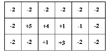
Computerized methods could be divided into two groups. First, heuristic algorithms, such as floated cone method, from which final the pit generated is not necessarily optimal. Second, , rigorous algorithms, such as Lerchs– Grossmann method, generated from which final pits are certainly optimal. The algorithm introduced here belongs to rigorous algorithms. Figure 1 shows a cross-sectional view of a hypothetical two dimensional economic block model containing eighteen blocks, which are square in shape. Expected economic value of each block is shown in center of blocks. Assuming a safe slope angle of 45 degree, before mining of any block in first second level, there are three overlying blocks in the first level, which must be removed. Similarly, before mining any block in the third level there are three overlying blocks in the second level and five overlying blocks in the first level that have to be removed.
Figure 1. A typical section from a 2D orebody model.
2. Algorithm for designing ultimate pit limits
131
proposed here and the FTA. The original FTA was introduced for production scheduling and determining the optimal sequence of extracting blocks. In FTA, it is assumed that the ultimate pit limits is known.
In the algorithm proposed here, positive blocks play a key role. The main logic in this method is that only positive blocks, which can pay costs of removing their overlying negative blocks, are capable of presenting in the final pit. Those costs may be paid either by positive block itself or jointly with other positive blocks that have the same overlying negative blocks. For mathematical formulation of this logic, a Linear Programming (LP) model was developed.
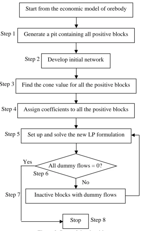
Figure 2 provides a schematic
representation of the steps involved in the algorithm.
Figure 2. Steps of the algorithm.
As shown, this algorithm is, indeed, an iterative network model. The steps are discussed below.
2.1. Setting initial network (Steps 1 and 2)
Firstly, the pit containing all the positive blocks is determined. Then a network is set on the blocks within that pit. In this network, blocks are represented by nodes and mining slope requirement is represented by the arcs. The arcs in the network represent the node precedence relationship within the pit. An arc is set from each positive value node to all the overlying negative value nodes in the cone of that block [13].
2.2. Assigning initial ranking coefficients to the positive value blocks (Steps 3 and 4)
Firstly, the cone value, CVi, of all positive value nodes within the network is determined. Then, a ranking coefficient is assigned to each of those nodes, according to the levels where they are located and their cone value. This process starts from second level. On the top most level, after level 1, where one or more positive value nodes exist, the node with the highest cone value is assigned to 1, and the second highest cone value node is assigned to 2, and so on. For instance, if there are 3 positive value nodes on that level, the node with the smallest cone value is assigned to 3. Then, the ranking process moves down one level. If there are some positive value nodes on that level, the node with the highest cone value is assigned to 4. Otherwise, a lower level is searched for positive value nodes. The process is performed for all the positive value nodes within the network. If two or more positive value nodes on the same level have the same cone value (tie condition), the coefficients are assigned randomly; two nodes must not be assigned the same coefficient [13]. These ranking coefficients will be used in LP problem formulation. [14]
2.3. The LP formulation to generate ultimate pit limits (Step 5)
Firstly, a dummy node D is added to network and is connected to all positive value nodes. This node, which assumed to have indefinite
Start from the economic model of orebody
Generate a pit containing all positive blocks
Develop initial network
Find the cone value for all the positive blocks
Assign coefficients to all the positive blocks
Set up and solve the new LP formulation
All dummy flows = 0?
Inactive blocks with dummy flows No
Yes
Stop Step1
Step2
Step 3
Step 4
Step 5
Step 7
132
positive value, prevents generating infeasible solutions. As mentioned later in the study, in each iteration, this dummy node causes some of positive value nodes to become inactive. Dummy node, like other positive value blocks, is assigned a ranking coefficient. This coefficient in the first iteration is the biggest coefficient within the network and in the next iterations is bigger than all active blocks’ coefficients. Amounts of flows in the arcs from positive value nods to negative value nodes are decision variables of the model.
The objective function of the model is minimizing arc connections in the network weighted by the assigned ranking coefficients. The objective function is expressed as:
, ,
,
Minimize
C
C
M
n m w n
i i j D D l
i j l
m w k j k j
f
f
f
(2)where Ci is the ranking coefficient for node i, for positive value nodes that are active in the network; n is number of all positive nodes in the network; m is number of positive nodes, which had become inactive in the previous iterations, so in the first iteration m is equal to zero; fi,j is the flow from node i to node j; j is
the index for the negative value nodes connected to the positive value node i with an arc coming from i; CD is coefficient of dummy node D, which is bigger than the last Ci, i.e. C n-m; fD,l is the dummy flow from node D to
positive node l; k is the index for positive inactive nodes; fk,j is the flow from node k to
node j; M is a big number that is bigger than CD.
If there are one or more positive value nodes on level 1, there is no need to include them in the formulation because there are no arcs formed from these nodes [13]. These nodes will be added to final pit derived from performing the algorithm.
The objective function is constructed in a way that the arcs will be set from high cone value nodes to support the negative nodes above them. In a given level, it is considered that the highest cone value node, say node i, has the highest chance of supporting all the negative value overlying it [13]. This arrangement causes the number of joint
supports (pay for a given negative value node by more than one positive value block) be minimized.
Furthermore, adding dummy node D to network prevents generating infeasible solutions, and setting its priority after active positive nodes causes the flow in dummy arcs to become non-zero, only when active positive nodes are unable to support removing their overlying negative nodes. The existing non-zero flow in an arc from node D to a given active positive node means that this node is unable to support negative nodes in its cone, and, thus, have to become inactive and set aside from the final pit.
The last term in the objective function involves positive nodes that have become inactive in the previous iterations. Setting their priority after node D prevent them helping active positive nodes for supporting joint negative nodes. In the first iteration, this term equals zero.
In ultimate pit limits problem, it is assumed that positive value nodes in the pit in order to be mined and processed and finally generate a profit, have to be capable to pay for removing their overlying negative nodes, by themselves or jointly with positive nodes having joint overlying negative nodes. Then, the flow capacity of positive nodes could not be less than what must be paid for upper levels negative nodes. A positive value node is limited in flow capacity to its value plus what receives from dummy node. Therefore, the constraint relating to a given positive node i, is expressed as:
, ,
w
D i i j i
j
f
f
V
(3) where Vi is the value of node i.On the other hand, each negative node in the final pit for removing requires enough flow from positive nodes in the lower levels. Therefore, the constraint relating to a given negative node j is calculated as:
, V
n
i j j
i
f
(4) where Vj is the negative value of node j and ε is a very small value.133
least equal to ε, which is strictly positive. ε is set to a very small number such as 0.001 that will not be ignored by the solver. Without using ε, if an overlying negative node is fully supported by an underlying positive value node, the total value of negative and positive nodes could be zero, without requiring a joint support. That generates zero value sub-pits, i.e. there may be a set of blocks in the final pit, which can be set aside without affecting pit value. This phenomenon violates the definition of ultimate pit limits mentioned in Section 1.
Note that if ε is set too high, the LP model might miss some positive value sub-pits, so the final pit would not be the most profitable pit. If the values of blocks are rounded to integer numbers, the total of the added ε values for all the overlying connected nodes should be kept below 1.
2.4. Controlling the algorithm (Steps 6-8)
The LP problem formulated in the previous section can be solved using a commercially available solver.
If the flow of any arc connecting dummy source to positive nodes, which were equal to zero in the previous iteration, changes , these positive nodes are inactivated, i.e. their coefficients are set equal to big M (bigger than coefficient of dummy node). Then, the next iteration starts and the model is solved with new coefficients.
On the other hand, if the flow of arcs connecting dummy source to positive nodes, which were equal to zero in the previous iteration, remains unchanged, the optimal pit is determined and the algorithm is terminated. The ultimate pit limits consist of positive nodes (the amount of arcs connecting dummy source to which in the all cycles remains equal to zero) and their cones, as well as all positive blocks in the first level, if any.
3. Application of the algorithm for a simple example
Application of the proposed algorithm is discussed using an example that can be considered as a cross-sectional view of some blocks on three consecutive elevations, or levels, shown in Figure 1.
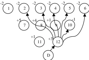
Firstly, the pit containing all the positive blocks is determined. Figure 3 shows this pit. The node identification number is written on the left top corner of each block, and the expected economic value of block is written at the center of each block. Then, a network is generated as shown in Figure 4. Since nodes 7, 8, 9, 11 and 12 have positive economic values, the arcs are set from these nodes to the nodes on the upper levels. For simplicity of the illustration, it is assumed that the blocks are the same in size and have to be mined with 45° slope angle in all directions.
Figure 3. Pit containing all the positive blocks.
A dummy source node, D, is added to the network. Node D is a positive node proposed to compensate for probable shortage in the positive nodes, in order to help them to support their overlying negative nodes. There are arcs between node D and all the positive nodes, as well as between positive nodes and the negative nodes in their cone. In Figure 4, only the arcs relating to node 12 are shown. These arcs show the precedence relationships of nodes based on the slope angle requirement. For example, in order to mine block 12, negative blocks 2, 3, 4, 5, 6 and 10 must be mined.
Figure 4. Network representation of the 2D block model shown in Figure 1; source node D is added.
1 2 3 4 5 6
7 8 9 10
11 12
D
-2 -2 -2 -2 -2 -2
+5 +4 +1 -1
134
In order to determine ranking coefficients, the cone value of all positive value nodes must be calculated. For example, for node 7,
CV7 = V7 + V1 + V2 + V3 =5 – 2 – 2 – 2 = –1.
Similarly, CV8 = – 2, CV9 = – 5, CV11 = 1,
CV12 = – 3.
Coefficients, Ci, are assigned to positive value nodes according to CVi value and the levels where nodes are located. In the second level, since CV7 is greater than CV8 and CV9,
then C7 is set to 1; and since CV8 > CV9, then
C8 and C9 are set to 2 and 3, respectively.
Similarly, in the third level, C11 is 4 and C12 is
5. The coefficient of dummy node in the initial formulation is the biggest one; therefore, CD =
6.
Now, according to section 2-3 the initial model can be formulated. This formulation and its solution are provided in Figure 5 and Table 1, respectively.
As given in Table 1, nodes 9 and 12, which have non-zero dummy arcs, are not capable for presenting in the final pit and have to become inactive. To inactivate these nodes, their coefficients in the LP formulation have to set big M, i.e. bigger than CD. Therefore, new
ranking coefficients of the positive nodes will be: C7 = 1, C8 = 2, C11 = 3, CD = 4, and both C9
and C12 can be set to 5.
min 7,1 7,2 7,3 2 8,2 8,3 8,4 3 9,3 9,4 9,5
4 11,1 11,2 11,3 11,4 11,5 5 12,2 12,3 12,4 12,5 12,6 12,10
6 ,7 ,8 ,9 ,11 ,12
Subject to ,12 12,2 12,3 12,4 12,5 12,6 12,10 3
f f f f f f f f f
f f f f f f f f f f f
fD fD fD fD fD
fD f
f f f f f f
1 ,11
1 ,9
4 ,8
5 ,7
1.001 , 2.001 , 2.001
12,10 12,6 12,5 11,5 9,5
2.001
12,4 11,4 9,4 8,4
12,3 11,3 9,3 8,3 7,3
11,1 11,2 11,3 11,4 11,5
9,3 9,4 9,5
8,2 8,3 8,4
7,1 7,2 7,3
D fD fD fD
f f f f f
f f f f
f f f f f
f f f f f
f f f
f f f
f f f
2.001
2.001 , 2.001
12,2 11,2 8,2 7,2 11,1 7,1
0 , 7, 8, 9,11,12, , 1, 2, ...,12 ,
f f f f f f
fi j i D j
Figure 5. Initial problem formulation.
Table 1. Solution of initial problem.
Variable Value Variable Value Variable Value Variable Value Variable Value
fD,12 0.002 f12,10 1.001 f11,5 1 f9,5 1.001 f8,4 0
fD,11 0 f12,6 2.001 f11,4 0 f9,4 0 f8,3 1.003
fD,9 0.001 f12,5 0 f11,3 0 f9,3 0 f8,2 2.001
fD,8 0 f12,4 0 f11,2 0 f7,3 0.998
fD,7 0 f12,3 0 f11,1 0 f7,2 2.001
135
min 7,1 7,2 7,3 2 8,2 8,3 8,4
3 11,1 11,2 11,3 11,4 11,5
4 ,7 ,8 ,9 ,11 ,12
5 12,2 12,3 12,4 12,5 12,6 12,10 5 9,3 9,4 9,5
f f f f f f
f f f f f
fD fD fD fD fD
f f f f f f f f f
Figure 6. Objective Function of second problem.
Now, the second iteration can begin. In the new problem formulation, objective function is changed according to the new ranking coefficients. But, constraints remain unchanged. New objective function and solution of new problem are provided in Figure 6 and Table 2, respectively.
As given in Table 2, amount of arc connecting dummy source to positive node 11,
fD,11, is non-zero. So, this node cannot be
presented in the final pit and has to become inactive. Therefore, its coefficients in the LP formulation must change to big M, i.e. bigger than CD, and new coefficients of the positive
nodes will be: C7 = 1, C8 = 2, CD = 3 and C12,
C9, and C11 can be set to 4.
Table 2. Solution of second problem.
Variable Value Variable Value Variable Value Variable Value Variable Value
fD,12 0.002 f12,10 1.001 f11,5 1.001 f9,5 1 f8,4 2.001
fD,11 0.001 f12,6 2.001 f11,4 0 f9,4 0 f8,3 0
fD,9 0 f12,5 0 f11,3 0 f9,3 0 f8,2 1.003
fD,8 0 f12,4 0 f11,2 0 f7,3 2.001
fD,7 0 f12,3 0 f11,1 0 f7,2 0.998
f12,2 0 f7,1 2.001
min 7,1 7,2 7,3 2 8,2 8,3 8,4 3 ,7 ,8 ,9 ,11 ,12
4 12,2 12,3 12,4 12,5 12,6 12,10 5 9,3 9,4 9,5
4 11,1 11,2 11,3 11,4 11,5
f f f f f f fD fD fD fD fD
f f f f f f f f f
f f f f f
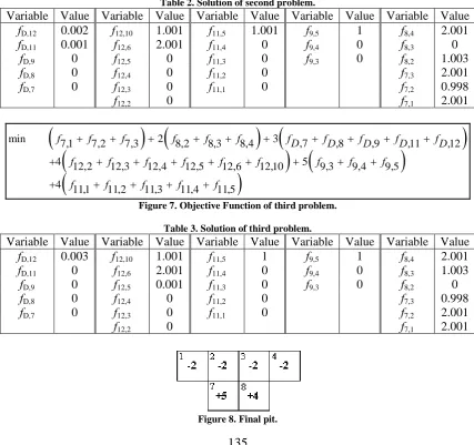
Figure 7. Objective Function of third problem. Table 3. Solution of third problem.
Variable Value Variable Value Variable Value Variable Value Variable Value
fD,12 0.003 f12,10 1.001 f11,5 1 f9,5 1 f8,4 2.001
fD,11 0 f12,6 2.001 f11,4 0 f9,4 0 f8,3 1.003
fD,9 0 f12,5 0.001 f11,3 0 f9,3 0 f8,2 0
fD,8 0 f12,4 0 f11,2 0 f7,3 0.998
fD,7 0 f12,3 0 f11,1 0 f7,2 2.001
f12,2 0 f7,1 2.001
136
Now, the third iteration can start. In the new problem formulation, the objective function will be changed according to new ranking coefficients. But, constraints will remain unchanged. New objective function and solution of new problem are provided in Figure 7 and Table 3, respectively.
Now, as given in Table 3, arcs between dummy source, D, and all active positive nodes from previous iteration, nodes 7 and 8, has remained zero. Therefore, the optimal pit is determined and the algorithm is terminated. Ultimate pit limits consist of the positive nodes 7 and 8 and their cones. Figure 8 shows the final pit.
4. Conclusions
In this paper, a linear programming model is developed to determine ultimate pit limits in open pit mining. This model, due to inherent LP problems, relies on a rigorous logic. So, the final generated pit is assumed to be optimal. Furthermore, it does not include any integer variables, so that it can solve large problems without running into time constraints.
By definition, ultimate pit limits is the smallest region within a mineralized area, which includes a set of blocks, the mining of which is technically feasible, and economically justified. The total value of blocks within that region is higher than every other set of mineable blocks.
Since profit is resulted from mining and processing positive value blocks, then positive blocks are the main reason and major base for any design, including final pit design, in the mining industry. Occurring non-positive value blocks within the pit is justified only if they overly positive blocks and prevent them from extracting, and underlying positive blocks are able to pay for removing them. This is the main logic behind the proposed algorithm and formulation. Indeed, this algorithm tests every positive value block within the ore-body if it can pay for removing negative blocks overlying it, by itself or jointly with other positive blocks having joint overlying negative blocks, or not. If a given positive block can do this job, it will remain in the final pit, otherwise must be left out.
References
[1]. Underwood, Robert, Tolwinski, Boleslaw,
1998. A mathematical programming
viewpoint for solving the ultimate pit
problem, European Journal of Operational
Research, 107, p.96-107.
[2]. Khalokakaie, R., Dowd, P. A., Fowell, R. J., 2000. Lerchs–Grossmann algorithm with
variable slope angles, Trans. Instit. Min.
Metall. (Sect. A: Min. technol.), 109, May– August 2000.
[3]. Lerchs, H., Grossmann, I. F., 1965.
Optimum design of open pit mines, CIM
Bull., 58, 1965, p.47–54.
[4]. Johnson, T. B., Barnes R. J., 1988.
Application of the maximal flow algorithm to
ultimate pit design, In Levary R. R. ed.
Engineering design: better results through operations research methods (Amsterdam: North Holland, 1988), p.518–31.
[5]. Yegulalp T. M., Arias J. A., 1992. A fast algorithm to solve the ultimate pit limit
problem, In Proc. 23rd symposium on the
application of computers and operations research in the mineral industries (APCOM) (Littleton, Colorado: AIME, 1992), p.391–7. [6]. Lemieux M., 1979. Moving cone
optimizing algorithm, In Weiss A. ed.
Computer methods for the 80s in the mineral industry (New York: AIME, 1979), p.329– 45.
[7]. Korobov S., 1974. Method for determining
optimal open pit limits (Montreal: Ecole
Polytechnique de l’Université de Montréal, 1974), 24 p. Technical report EP74-R-4 [8]. Dowd P. A., Onur A. H., 1993. Open-pit
optimization—part 1: optimal open-pit
design, Trans. Inst. Min. Metall. (Sect. A: Min. industry), 102, 1993, p.A95–104. [9]. Wilke F. L., Wright E. A., 1984.
Determining the optimal ultimate pit design for hard rock open pit mines using dynamic
programming, Erzmetall, 37, 1984, p.139–
44.
137
[11]. Matheron G., 1975. Paramétrage des
contours optimaux (Fontainebleau: Centre de
Géostatistique et de Morphologie
mathématique, 1975), 54 p. Internal report N-403; Note géostatistique128.
[12]. François-Bongarçon D., Guibal D., 1982. Algorithms for parameterizing reserves
under different geometrical constraints, In
Proc. 17th symposium on the application of computers and operations research in the
mineral industries (APCOM), (New York: AIME, 1982), p.297–309.
[13]. Ramazan, Salih, 2006. The new Fundamental Tree Algorithm for production
scheduling of open pit mines. European
Journal of Operational Research.
[14]. Hustrulid, W., Kuchta, M., 1995. Open
Pit Mine Planning & Design, A.A.Balkema,