© Shiraz University
A Hybrid Approach Based on Numerical, Statistical and Intelligent Techniques for Optimization of Tube Drawing Process to
Produce Squared Section from Round Tube
M. Ghasempour-Mouziraji1*, M. Hosseinzadeh2, M. Bakhshi-Jooybari3 and J. Maktoubian
1Department of engineering, Islamic Azad university of Sari, Sari, Iran.
2Department of engineering, Ayatollah Amoli Branch, Islamic Azad university, Amol, Iran. 3Department of Mechanical engineering, Babol Noshirvani University of Technology, Iran. 4International School of Information Management (ISIM), University of Mysore, Mysore, India.
Abstract: In tube drawing process, there is a bunch of parameters playing key roles in the process performance. Thus finding the optimized parameters is a controversial issue. The current study aimed to produce a squared section of round tube by tube sinking process. Finite element method (FEM) was used to simulate the process. Then, to find a meaningful kinship between process input and output parameters the developed FE model was associated with the design of an experiment based on response surface methodology (RSM). The sufficiency of each model was checked by analyzing the variances. Further, the SA (simulated annealing) was associated with RSM models to find the optimal solution regarding maximum thickness distributions and minimum force and dimensional error. Hereafter, for performing accurate optimization, principal component analysis was used to find the appropriate weight factor of each response. The obtained results were in right congruence with those derived from the simulation and confirmatory experiment.
Keywords: Tube sinking, square sections, Multi-objective optimization.
1. Introduction
Polygonal tubes are widely used in various engineering and industrial applications to produce lightweight structures [1]. There are four main methods used to produce tubes, namely tube sinking, tube drawing with fixed mandrel, tube drawing with floating mandrel and tube drawing with movable mandrel. In tube sinking process, the tubes are pulled out through the die with no underlying support, and the tube’s diameter decreases and its thickness remains constant but it might increase on some occasions. Having low surface quality is the main disadvantage of this method. Bayoumi et al [2] produced polygonal tubes by using rollers which are shapely-located. The roller’s radius, thickness, section shape and friction coefficient were investigated to find the drawing force in this process.
In tube drawing with fixed mandrel, the primary tube is drawn after being placed on the mandrel. Thickness and diameters decrease but both inner and outer surfaces are good in quality. Mandrels could have different shapes due the desired shape of the tube and also they play key roles in the dimensional accuracy of the produced tubes. The high rate of friction between the tubes and mandrel leads the low accuracy of the produced tubes due to the corrosion between them. As previously mentioned, fixed mandrels are associated with some problems but tube drawing with floating mandrel has tackled this task. The cone-shaped mandrel is constant in the deformation zone which has contact with the inner surface of the tube, and the balance between the compressive and frictional forces in this location remains constant.
In tube drawing with movable section, the mandrel is located in the primary tube and passes through the die with the tube. The goals of this process are to decrease the thickness and increase the length of the tube. Numerous researches in shaping round tubes have been carried out by many researchers. The production of rectangular tubes by using hydroforming expansion has been compared with combined hydraulic expansion and hydroforming [3]. Manabe and Amino have already investigated on circular tubes into square tubes [4]. Kridli et al [5] carried out the die geometry and material property in producing square tubes by using hydroforming considering two-dimensional plane strain FE code. Experimental and numerical investigations of tube drawing with various thicknesses were conducted by Bihamta et al [6]. Leu et al [7] designed a die which was able to prevent fracture by using damage criteria. Boton et al [8] developed a model for tube drawing with fixed mandrel by using numerical and mathematical formulae. MSC.SUPERFORM was used in this research, then the numerical and experimental results were compared. Finally, they found that, 7-10 die half angle was the most suitable angle for drawing, and that condition plays a key role in this process. Karenzis et al [9] developed a model for cold tubes which are sensitive to thermal variation. Residual stress, tension force, and the efficiency of the process were investigated via ABAQUS. Production of thin tubes which are used in medical applications was studied by Yushida et al [10]. They used titanium material and MARC software in their research. They have found that tube sinking has the highest thickness increase among different methods of tube drawing. Also, various studies have been carried out to optimize the manufacturing process by using statistical methods in machining [11, 12], welding [13, 14], metal forming [15, 16], coating [15, 16] and etc. Therefore, the method has found applicability to the problems and could be applied in modeling and optimization of tube drawing process. Many researches have employed RSM to optimize different processes, such as tube drawing process which was used to produce square-shaped tubes by M. Hosseinzadeh et al. [17]. They optimized tube drawing process parameters such as entrance velocity, bearing length, friction coefficient, and die angle by using FE simulation and experimental test. The central composite design matrix was used for achieving optimum parameters. M. Salehi et al [18] utilized DOE (design of experiment), RSM and artificial bee ant colony algorithm to optimize the parameters of rectangular tubes. They investigated the effects of the parameters on geometrical error, thickness distribution and drawing force. Mirshaban Jafari et al [19] optimized the spring back phenomenon in deep drawing process by using ANFIS to attain the least spring back.
results which have been achieved by FE simulation. One key factor that should be considered in multi-objective optimization is finding adequate weight of each response that has been achieved in this research by PCA (principal component analysis). Simulated annealing algorithm is used to integrate the RSM model and achieve weight factor by using singular objective function. It is worth notifying that singular objective function is derived from weighted function for each factor (force, MSE, thickness) to reach a sole and target function in order to proceed the optimization. Lastly, once the optimal results found, the data are validated through experimental and simulation results. The current study is classified into seven steps that can be seen in this section.
1.Finding the mechanical properties of the material running FE simulation
2. Validating the FE result by performing experimental tests (choosing the same condition in the
simulation and experiments)
3. Creating a statistic model of each response with RSM
4. Using ANOVA to check the sufficiency of the model
5. Obtaining weight factor of each response through PCA and developing a singular objective
function
6. Utilizing simulated annealing to optimize objective function and draw out the results which have
been optimized
7. Using FE model and experimental tests to confirm the achieved results
2. Experimental Steps
Pure copper tubes have been utilized for running the experimental tests and FE model. Also, tension test has been used based on ASTM-A370 standard to find the mechanical properties of copper tubes. The sample
was considered as a deformable pure copper tube with the stress-strain relationship of ϭ=402ɛ0.32 MPa where
402 MPa is strength coefficient and 0.32 is strain hardening exponent which was determined experimentally using tensile test data. It is worth notifying that the tube’s thickness is 0.75 mm and the inner diameters is 11.2. Table 1 elucidates the mechanical properties of the tubes.
Table 1. Mechanical properties of pure copper. Density
(kg/m3) Yield strength (MPa) Ultimate tensile strength (MPa) Young modulus (GPa) coefficient Poisson
8900 180 270 110 0.343
A hand-made drawing machine with 3KW capacity has been used to run the experimental tests. The drawing machine was equipped with an inverter to control the velocity which should be used in this process. To perform the drawing process, the tube is drawn through the die with a series of chains.
Figure 1a illustrates the drawing machine with the dies and Fig. 1c depicts various parameters of the process. It is worth notifying that, the length of the sides in the dies is 9 mm.
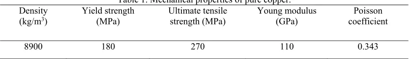
One of the most important and challenging issues in tube sinking process to produce square section is corner fillets which deteriorate dimensional accuracy. It can be mentioned that there is difference between the produced tubes and the ones anticipated (Fig. 2). In addition, another parameter which plays a key role in shape and dimensional accuracy is springback. The dimensional accuracy has been measured by VMM (video measurement machine) and MSE (mean square error) equation which is shown here
n
i e o
d d N MSE
1
2
) ( 1
In MSE equation, N, deand do are the numbers of measurement points on drawn section, anticipated
and achieved dimensions, respectively. The thickness distribution was measured in 30 points by digital micro meter in two paths which one is linear and the other is peripheral.
Fig. 1. Experimental setup (a) details of the drawing machine (b) Square dies with different input angles and various parameters of the process.
Fig. 2. calculation of MSE and its schematic view
3. Finite Element Simulation
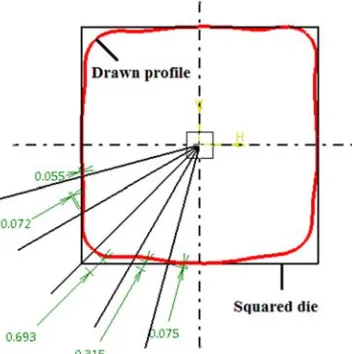
because it has no conspicuous deformation compared with the tube that has been modeled as a deformable body by C3D8R. Different friction models can be used in simulation via ABAQUS, but in the current study surface to surface model was utilized. The velocity and symmetry boundary conditions have been used to model the movement of the tube and fix the die. Three friction coefficients were used in simulation according to different lubricants, SAE 10, sunflower oil and grease which were considered 0.1, 0.2 and 0.3, respectively. Tension test has been employed to achieve the pure copper property which has 99.9 purity. One of the most controversial issues in tube drawing process is the thermal effect that should be considered but in this research, it has been ignored due to the drawn tube’s temperature. Drawn tube’s temperature was measured by a thermocouple and the highest temperature was 70°c which due to the melting temperature of the pure cupper, it was about %7[1,2,6].
Fig. 3. Finite element modelling of tube drawing and its definition.
3.1. FE Model’s validation
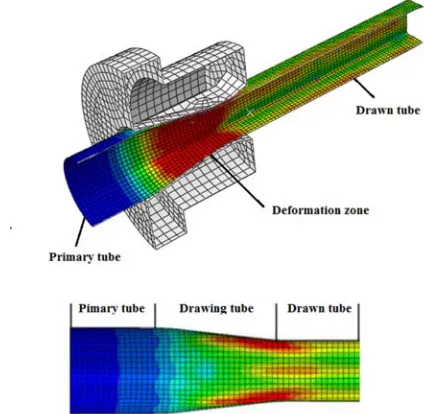
FE model of the process has been validated with experimental results, namely dimensional accuracy and thickness distribution. As can be seen in Fig. 4, there is adequate correlation between the experimental and numerical results.
The accuracy of FE model has been analyzed with thickness distribution in two paths, linear and peripheral. Figure 5 depicts both linear and peripheral paths and it can be found that there is good correlation between the experimental and FE results.
Fig. 5. Thickness distribution along two directions.
4. Designing the Experiment and Developing RSM Models
4.1. Construction design matrix
In the previous section, the accuracy of FE results was validated and it could be useful to anticipate the characteristic which is one of the main goals of the current research. However, it takes much more time, several hours, to run all simulation. RSM is a more suitable method for anticipation and has been used in this research to find the correlation between tube sinking parameters and process responses (Drawing force, MSE, and thickness distribution). Data have been collected based on simulations and design of experiment (DOE). Input parameters are die half angle, friction coefficient and bearing length and have been considered in three levels which are shown in Table 2. 81 experiments are required to run full factorial design which is calculated according to N=Lm formula that N, L and m are the numbers of possible design, level of each factor and number of factor, respectively. Five factors-three levels face-centered central composite design has been employed to reach additional reduction. To achieve this goal, 25 are required to gather the data for
0.5 0.7 0.9 1.1 1.3
0 2 4 6 8 10
Li
near
th
ickness
d
ist
ribut
io
n
(m
m)
Distance from initial poin (mm) Experiment
0.6 0.8 1 1.2 1.4
0 2 4 6 8 10 12
Per
ipheral
th
ickn
ess
(m
m
)
Distance from initial point (mm) (b)
running RSM. For testing the adequacy of the model, analysis of variance (ANOVA) has been used. Design matrix and achieved values have been depicted in Table 3.
Table 2. Process factors and their levels.
Factors Symbol Unit Level 1 Level 2 Level 3
Die angle α deg 2.5 5 7.5
Deformation length L mm 2 4 6
friction coefficient µ - 0.1 0.2 0.3
Drawing velocity V mm/min 5 7.5 10
Table 3. Face centered central composite design matrix and obtained values of responses. No
α (deg) (mm) L µ V (mm/min) Force (N) thickness linear (mm)
peripheral thickness
(mm) MSE
1 2.5 2 0.1 5 8888.95 0.9465 1.2750 0.3812
2 7.5 2 0.1 5 5211.44 0.9434 1.2795 0.3564
3 2.5 6 0.1 5 8533.22 1.2346 0.9500 0.3785
4 7.5 6 0.1 5 4959.68 0.9458 1.2859 0.4941
5 2.5 2 0.3 5 21727.9 0.9458 1.2535 0.1726
6 7.5 2 0.3 5 10567.3 0.9324 1.2779 0.3092
7 2.5 6 0.3 5 20778.3 0.9493 1.2304 0.1734
8 7.5 6 0.3 5 9457 0.9539 1.2853 0.3739
9 2.5 2 0.1 10 8910.56 0.9460 1.2788 0.3991
10 7.5 2 0.1 10 5228.94 0.9452 1.2691 0.4639
11 2.5 6 0.1 10 8497.99 0.9500 1.2363 0.4091
12 7.5 6 0.1 10 4964 0.9536 1.2901 0.5021
13 2.5 2 0.3 10 21852.1 0.9471 1.2612 0.1504
14 7.5 2 0.3 10 10551.7 0.9377 1.2748 0.3103
15 2.5 6 0.3 10 20700 0.9502 1.2333 0.1746
16 7.5 6 0.3 10 9391 0.9555 1.2897 0.3746
17 2.5 4 0.2 7.5 14981.6 0.9490 1.2328 0.2365
18 7.5 4 0.2 7.5 7595.85 0.9496 1.2692 0.4123
19 5 2 0.2 7.5 9281.6 0.9414 1.2632 0.3832
20 5 6 0.2 7.5 9270.14 0.9334 1.2774 0.3900
21 5 4 0.1 7.5 5951 1.2804 0.9391 0.4836
22 5 4 0.3 7.5 12639.2 1.2821 0.9395 0.2712
23 5 4 0.2 5 9216.66 1.2924 0.9436 0.3873
24 5 4 0.2 10 9256.47 1.2745 0.9499 0.3897
25 5 4 0.2 7.5 9250.72 1.2726 0.9442 0.3915
4.2. Development of RSM model for each response
As previously-mentioned, RSM has been used to discover the correlation between the parameters. When the effects of the parameters were studied, then the mathematical model, second-order polynomial was developed which is shown in Eq. (2).
ju k
i ij iu iu
k
i ii iu k
i i
X X b X b X b b
Y
1
2 1 1
0 (2)
In Eq. (2), Y is response (peripheral thickness and linear thickness distribution, MSE and drawing force) and coefficient, variable, experiment number, factor number, higher order term of variable and interaction terms are shown by b0, bi, bii and bij, Xiu (V, L, α, and µ), u(1-15), k(1-4), Xiu2 and Xiu, Xju, respectively.
4.2.1. RSM model of responses
By using design expert and the data which have been achieved from Table 3, effects of parameters have been calculated by considering Eq. (2) constants. Equation (3-6) depict the mathematical relationship of responses.
2 2 2 2 873 . 5 7 . 2182 649 . 0 47 . 322 97 . 10 03 . 4 9 . 964 92 . 0 16 . 765 028 . 1 31 . 111 05 . 83860 44 . 55 33 . 3178 5 . 8075 V L V LV L V L V L Force (3) MSE’s equation 2 3 2 3 2 3 2 3 3 3 3 10 26 . 7 10 83 . 3 10 36 . 5 057 . 0 011 . 0 10 98 . 3 10 82 . 1 10 61 . 5 028 . 0 017 . 0 10 17 . 8 087 . 0 019 . 0 062 . 0 39 . 0 V L V LV L V L V L MSE (4)
Thickness distribution’s equation
2 2 2 2 3 3 3 01 . 0 15 . 10 06 . 0 03 . 0 07 . 0 10 52 . 3 08 . 0 10 99 . 2 06 . 0 10 1 . 3 27 . 0 78 . 4 551 . 0 338 . 0 808 . 0 V L V LV L V L V L Linear (5) 2 2 2 2 3 3 3 01 . 0 65 . 9 058 . 0 034 . 0 06 . 0 10 75 . 3 097 . 0 10 05 . 3 05 . 0 10 85 . 5 23 . 0 411 . 4 55 . 0 32 . 0 53 . 1 V L V LV L V L V L Peripheral (6)
4.2.2. Is the developed model adequate?
The adequacy of the experiential relationship has been checked by using ANOVA and the results are shown in 4-7 tables. In the current study, the significance of the experiential relationship has been checked by considering F and probability values. Also, the influence of each factor on the responses has been assessed by using F-values. The sufficiency of fit for the model has been shown by the value of (R2 > 0.99). Good correlation can be seen between the anticipated and adjusted R2. Tables 4-7 show the value of probability > F for the experiential relationship which is less than 0.05. As can be seen, lack of fit was not significant for the model [11].
Table 4. ANOVA for drawing force. Source Sum of
Squares
Degree of Freedom
Means of Square
F-Value Prob>F Significance
Model 6.64×10⁸ 14 4.74×10⁷ 340.85 <0.0001 Significant
α 2.49×10⁸ 1 2.49×10⁸ 1788.58 <0.0001
L 1.78×10⁶ 1 1.78×10⁶ 12.83 0.0027
µ 3.25×10⁸ 1 3.25×10⁸ 2336.81 <0.0001
V 8.42 1 8.42 6.04×10⁻⁵ 0.9939
αL 423.3 1 423.3 3.041×10⁻³ 0.9567
αµ 5.86×10⁷ 1 5.86×10⁷ 421.1 <0.0001
αV 529.69 1 529.69 3.8×10⁻³ 0.9516
Lµ 5.95×10⁵ 1 5.95×10⁵ 4.28 0.0562
LV 6517.3 1 6517.3 0.047 0.8316
µV 120.45 1 120.45 8.65×10⁻⁴ 0.9769
α2 1.05×10⁵ 1 1.05×10⁵ 75.61 <0.0001
L2 17.47 1 17.47 1.255×10⁻⁴ 0.9912
µ2 1234.36 1 1234.36 8.86×10⁻³ 0.9262
V2 3491.19 1 3491.19 0.025 0.8763
Residual 2.08×10⁶ 15 1.39×10⁵ - -
Lack-of-fit 2.08×10⁶ 10 2.08×10⁵ 3.57 0. 8652 Insignificant
Table 5. ANOVA for linear thickness distribution.
Source Sum of Squares Degree of Freedom Means of Square F-Value Prob>F Significance
Model 0.69 14 0.049 12.25 <0.0001 Significant
α 5.064×10⁻³ 1 5.064×10⁻³ 1.26 0.2790
L 6.45×10⁻³ 1 6.45×10⁻³ 1.61 0.2233
µ 4.72×10⁻³ 1 4.72×10⁻³ 1.18 0.2944
V 4.48×10⁻³ 1 4.48×10⁻³ 1.12 0.3062
αL 3.86×10⁻³ 1 3.86×10⁻³ 0.96 0.3415
αµ 4.76×10⁻³ 1 4.76×10⁻³ 1.19 0.2924
αV 5.6×10⁻³ 1 5.6×10⁻³ 1.4 0.2550
Lµ 4.13×10⁻³ 1 4.13×10⁻³ 1.03 0.3257
LV 4.98×10⁻³ 1 4.98×10⁻³ 1.24 0.2821
µV 5.06×10⁻³ 1 5.06×10⁻³ 1.27 0.2783
α2 0.14 1 0.14 34.36 <0.0001
L2 0.15 1 0.15 38 <0.0001
µ2 0.027 1 0.027 6.68 0.0207
V2 0.028 1 0.028 6.97 0.0185
Residual 0.06 15 4×10⁻³ - -
Lack-of-fit 0.06 10 6×10⁻³ 0.074 0. 1119 Insignificant
R2=0.9915 R2adjusted=0.9445 R2predicted=0.9637
Table 6. ANOVA for peripheral thickness distribution.
Source Sum of Squares Degree of Freedom Means of Square F-Value Prob>F Significance
Model 0.67 14 0.048 12.24 <0.0001 Significant
α 0.018 1 0.018 4.6 0.0487
L 6.99×10⁻³ 1 6.99×10⁻³ 1.78 0.2015
µ 3.25×10⁻³ 1 3.25×10⁻³ 0. 83 0.3769
V 5.07×10⁻³ 1 5.07×10⁻³ 1.29 0.2733
αL 0.014 1 0.014 3.49 0.0812
αµ 3.45×10⁻³ 1 3.45×10⁻³ 0.88 0.3625
αV 5.35×10⁻³ 1 5.35×10⁻³ 1.49 0.2414
Lµ 6.058×10⁻³ 1 6.058×10⁻³ 1.55 0.2330
LV 5.62×10⁻³ 1 5.62×10⁻³ 1.43 0.2496
µV 4.62×10⁻³ 1 4.62×10⁻³ 1.18 0.2946
α2 0.12 1 0.12 30.58 <0.0001
L2 0.14 1 0.14 36.32 <0.0001
µ2 0.024 1 0.024 6.16 0.0254
V2 0.021 1 0.021 5.25 0.0369
Residual 0.059 15 3.92×10⁻³ - -
Lack-of-fit 0.059 10 5.88×10⁻³ 0.085 0. 2439 Insignificant
R2=0.9932 R2adjusted=0.9425 R2predicted=0.9648 Table 7. ANOVA for mean square error.
Source Sum of Squares Degree of Freedom Means of square F-Value Prob>F Significance
Model 0.25 14 0.018 43.66 <0.0001 Significant
α 0.07 1 0.070 169.99 <0.0001
L 6.57×10⁻³ 1 6.57×10⁻³ 16 0.0012
µ 0.13 1 0.13 328 <0.0001
V 1.2×10⁻³ 1 1.2×10⁻³ 2.93 0.1076
αL 4.64×10⁻³ 1 4.64×10⁻³ 11.3 0.0043
αµ 0.013 1 0.013 30.58 <0.0001
αV 5.04×10⁻⁴ 1 5.04×10⁻⁴ 1.23 0.2856
Lµ 5.32×10⁻⁵ 1 5.32×10⁻⁵ 0.13 0.7238
LV 2.54×10⁻⁴ 1 2.54×10⁻⁴ 0.62 0.4437
µV 2.098×10⁻³ 1 2.098×10⁻³ 5.1 0.0392
α2 8.73×10⁻³ 1 8.73×10⁻³ 20.36 0.0004
L2 7.45×10⁻⁵ 1 7.45×10⁻⁵ 0.18 0.6763
µ2 3.81×10⁻⁵ 1 3.81×10⁻⁵ 0.093 0.7648
V2 1.36×10⁻⁴ 1 1.36×10⁻⁴ 0.33 0.5727
Residual 6.16×10⁻³ 15 4.11×10⁻⁴ - -
Lack-of-fit 6.16×10⁻³ 10 6.165×10⁻⁴ 0.091 0. 4891 Insignificant
5. Optimization Process
5.1. Utilizing PCA to find a suitable weight factor for each response
In optimization process, the weight of each factor should be determined according to importance and in the current research principal component analysis (PCA) has been used to reach this goal. It is worth notifying that PCA is a series of statistical analyses which are employed to observe the importance of the quality of each character. Information overlap and internal correlation occur in multivariate research due to the number of variables. In these cases, PCA could be useful to address this issue by reducing the dimension to detect uncorrelated factors. More information about the PCA is found in references [10, 11]. In table 8 the evaluation of the correction coefficient matrix and characterization of the corresponding values have been shown. The eigenvector corresponding to each eigenvalue is listed in Table 9. Table 10 illustrates the contributions of DF, LTD, PTD and MSE which are 0.2287, 0.2841, 0.2501 and 0.2372, respectively.
Table 8. Eigenvalues and explained variations for principal component. Principal component Eigenvalues Explained variations (%)
First 0.0061 0.15
Second 0.0488 1.22
Third 1.6975 42.43
Fourth 2.2476 56.19
Table 9. Eigenvectors for principal component. Quality
characteristics
Eigenvectors
first principal
component second principal component third principal component fourth principal component
DF -0.203 -0.7064 -0.5215 -0.4782
LTD -0.7105 -0.011 -0.4595 0.5330
PTD -0.7025 -0.0149 0.5061 -0.5001
MSE 0.0362 -0.7077 0.5106 0.4870
Table 10. The contribution of each individual quality characteristic for the fourth principal component. Quality characteristics Contribution
DF 0.2287
LTD 0.2841
PTD 0.2501
MSE 0.2372
5.2. Creation of objective function
Multi-criteria problem has been converted to a single criterion task due to multi-objective optimization approach. Equation (6) shows the objective function.
E MS D
PT ˆ w ˆ
w LTD w DF w
F 1 ^ 2 ^ 3 1 (6)
Where w1, w2, w3 and w4 are the weighting factors that are related to each output which was obtained
through principal component analysis. ^
DF,LTD^ , PTD^ and MSE^ are the normalized values of DF, LTD, PTD and MSE that were achieved
by the following equations:
min max
min ^
D D
D D DF
F F
F F
(7)
min max
min ^
L L
L L LTD
TD TD
TD TD
(8)
min max
min ^
PTD
PTD PTD
PTD PTD
min max
min ^
MSE
MSE MSE
MSE MSE
(10)
I should hasten to add that, "min" and "max" are signs of minimum and maximum values of given parameters, indexless term is the quality characteristic which has been obtained from RSM. Simulated annealing algorithm is used for minimization aims, which is the key reason that LTD and PTD were shown by a minus sig. The constructed objective function (i.e. Eq. (6)) is associated with simulated annealing algorithm and optimization is performed.
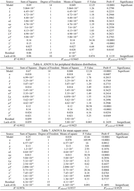
5.3. Utilizing SA to find the optimal combination and results validation
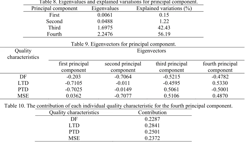
The flowchart of SA and its procedure, shown in Fig. 6, are aimed to reach the optimal solution. Same as the other evolutionary algorithms, SA requires its own parameters which should be carried out. The requirement for carrying SA algorithm has been shown in Table 11.
MATLAB software has been used for developing SA code but prior to utilizing this code, it had been checked by some optimization’s function, namely Rastrigin and Rosenbrock, the results have shown that the results are able to discover the optimal results with high accuracy.
Table 11. SA’S setup parameters [12]. Parameter Value/function Remark
X0 [0 0 0 0] Initial point Tinit 500 Initial temperature
H(X) Eq. 6 Objective function which uses normalized RSM models along with their related weight factors
R X=rand(4,1) Random vector X in the range of [0,1]
kB 1 Boltzmann constant
ST 10e-8 Stop temperature
C 0.9 Cooling rate
N 300 Maximum number of tries within one temperature
The optimal solution which has been achieved through simulated annealing has been shown in Table 12. Ten runs have been done to check the accuracy of the algorithm. Afterward, experimental and numerical runs have been carried out by considering the optimal combination. The results show the comparison of experimental, FE and RSM-SA in Table 13. It can be seen that there is adequate correlation, 95% for FE and 90% for experimental, between the confirmatory tests. Eventually, it is argued that the offered method has accuracy and could be used in tube sinking’s optimization. Also, it could be utilized in the other manufacturing process to swell the number of experiments and cost.
Table 12. Optimal parameter combination achieved from simulated annealing.
α (deg) µ V
(mm/min) L (mm) DF (N) (mm) LTD (mm) PTD MSE
7.49 0.28 5.01 3.03 10112.13 1.09 1.1 0.3184
Table 13. Experimental, FE and RSM-SA optimal results comparison.
Characteristic RSM-SA FE simulation Experiment
Drawing force (N) 10112.13 9667.2 9384.057
Linear thickness (mm) 1.09 1.046 1.0148
Peripheral thickness
(mm) 1.1 1.064 1.0318
Mean square error 0.3184 0.3032 0.02997
6. Conclusion
In this present work, an integrated approach including numerical, statistical and evolutionary techniques was proposed for the optimization of tube sinking process in fabricating square sections from round tubes. Firstly, ABAQUS/EXPLICIT software has been employed to develop the tube sinking of pure copper. In the next step, FE results have been validated with experimental results. Afterward, a series of runs, 25 FE run, have been implemented based on CCD design matrix to achieve the data to develop RSM models. Adequacies of MSE, drawing force linear and peripheral thickness distribution were performed by analyzing the variances, and the high R2 value implied that the RSM models have sufficient correlation between experimental and numerical results. Combination of FE model and RSM could be useful in predictingthe tube sinking process. In addition, this combination has reduced the number of experimental tests which are really time-consuming processes. Next, appropriate weight factor has been analyzed by using PCA for constructing objective function. In the last step, the optimum parameters have been found by using RSM-SA. Optimization process aimed to minimize the drawing force and MSE and maximize the linear and peripheral thickness distribution. The combination of die angle of 7.5 deg, friction coefficient of 0.3, entrance velocity of 5 mm/min and bearing length of 3 mm is the desirable result which could be achieved. This optimal combination has been confirmed through one additional run and another experimental test. According to what has been found in the current research, it can be mentioned that the combination of RSM
7. References
[1] L.S. Bayoumi, A.S. Attia, Determination of the forming tool load in plastic shaping of a round tube into a square tubular section. J Mater Process Technol 209(2009) 1835-1842.
[2] L.S. Bayoumi, Cold drawing of regular polygonal tubular sections from round tubes, Int J Mech Sci 43(2001) 241-253.
[3] Y.M. Hwang, Y. Altan Finite element analysis of tube hydroforming processes in a rectangular die, Fini Ele in Analys Des 39(2002)1071-1082.
[4] K. Manabe, M. Amino, Effects of process parameters and material properties on deformation process in tube hydroforming. J Mater Process Technol 123(2002) 285-291.
[5] G.T. Kridli, L. Bao, P.K. Malliek, Y. Tian, Investigation of thickness variation and corner filling in tube hydroforming, J Mater Process Technol 133(2003) 287-296.
[6] R. Bihamta, Q.H. Bui, M. Guillot, G. D’Amours, A. Rahem, M. Fafard, A new method for production of variable thickness aluminium tubes: Numerical and experimental studies, Journal of Materials Processing Technology
211(2011) 578–589.
[7] D.K. Leu, J.Y. Wu, Finite element simulation of the squaring of circular tube, Int J Adv Manuf Technol 25(2005) 691-699.
[8] F.O. Neves, T. Buttons, C. Caminaga, F.C. Gentile, Numerical and experimental analysis of tube drawing with fixed plug (2005).
[9] P. Karnezis, D.C.J. Farrugia, Study of cold tube drawing by finite-element modeling, Journal of Materials Processing Technology 80(1998) 690–694.
[10]K. Yoshida, H. Furuya, Mandrel drawing and plug drawing of shape-memory-alloy fine tubes used in catheters and stents, Journal of Materials Processing Technology, 153(2004) 145–150.
[11]M. Ghasemi-Baboly, M. Aminian, Z. Leseman, R. Teimouri, Application of soft computing techniques in modeling and analysis of MRR and Taper in laser machining process as well as weld strength and weld width in laser welding process. Soft Comput, DOI 101007/S00500-014-1305-x, (2104).
[12]Vazini Shayan, R. Azar Afza, R. Teimouri, Parametric study along with selection of optimal solutions in dry wire cut machining of cemented tungsten carbide (WC-Co). J Manuf Proc 15(2013) 644-658.
[13]S. Parsa Khanghah, M. Bouzarpoor, M. Lotfi, R. Teimouri, Optimization of micro-milling parameters regarding burr size minimization via RSM and simulated annealing algorithm. Transaction of the Indian Institute of Metal, DOI 10.1007/s12666-015-0525-9.
[14]H. Sohrabpoor, S. Parsa Khanghah, R. Teimouri. Investigation of lubricant condition and machining parameters while turning of AISI 4340. Int J Adv Manuf Technol. DOI 1 0.1007/s00170-014-6395-1, (2105).
[15]Y. Rostamiyan, A. Seidnaloo, H. Sohrabpoor, R. Teimouri, Experimental studies on ultrasonically assisted friction stir spot welding of AA6061. Arch Civil Mech Eng. DOI: 10.1016/j.acme.2014.06.005.
[16]M. Ahmadnia, A. Seidanloo, R. Teimouri, Y. Rostamiyan, K.H. Tirtashi, Determining influence of ultrasonic assisted friction stir welding parameters on mechanical and tribological properties of AA6061 joints. Int J Adv Manuf Technol. DOI 1 0.1007/s00170-015-6784-0, (2015).
[17]M. Hosseinzadeh, M. Ghasempour Mouziraji, An analysis of tube drawing process used to produce squared sections from round tubes through FE simulation and response surface methodology, The International Journal of Advanced Manufacturing Technology 87.5-8 (2016) 2179-2194.
[18]M. Salehi, M. Hosseinzadeh, M. Elyasi, A study on optimal design of process parameters in tube drawing process of rectangular parts by combining box–behnken design of experiment, response surface methodology and artificial bee colony algorithm, Transactions of the Indian Institute of Metals 69.6 (2016) 1223-1235.
ﻴﻟﺎﻧآ ﺮﺑ ﻲﻨﺘﺒﻣ ﻲﺒﻴﻛﺮﺗ دﺮﻜﻳور
ﺰ
ﺪﻨﻳآﺮﻓ يزﺎﺳ ﻪﻨﻴﻬﺑ ﺖﻬﺟ ﺪﻨﻤﺷﻮﻫ شور و يرﺎﻣآ ،يدﺪﻋ
يوﺮﻳاد ﻊﻄﻘﻣ زا ﻲﻌﺑﺮﻣ ﻊﻄﻘﻣ ﺎﺑ ﻪﻟﻮﻟ ﺪﻴﻟﻮﺗ رد ﻪﻟﻮﻟ ﺶﺸﻛ
ﻲﺟﺮﻳزﻮﻣ
رﻮﭙﻤﺳﺎﻗ
ناﺮﻬﻣ
1
*،
هداز
ﻦﻴﺴﺣ
ﻲﻀﺗﺮﻣ
،
2
ﻲﺸﺨﺑ
ﺪﻤﺤﻣ
،
3
نﺎﻴﺑﻮﺘﻜﻣ
لﺎﻤﺟ
،
4
1 سﺎﻨﺷرﺎﻛ ناﺮﻳا ،يرﺎﺳ ﺪﺣاو ﻲﻣﻼﺳا دازآ هﺎﮕﺸﻧاد ،ﻲﺳﺪﻨﻬﻣ هﺪﻜﺸﻧاد ،ﻚﻴﻧﺎﻜﻣ ﺪﺷرا
.
2 ناﺮﻳا ،ﻲﻠﻣآ ﷲا ﺖﻳآ ﺪﺣاو ﻲﻣﻼﺳا دازآ هﺎﮕﺸﻧاد ،ﻲﺳﺪﻨﻬﻣ هﺪﻜﺸﻧاد ،رﺎﻳدﺎﺘﺳا .
3 ناﺮﻳا ،ﻞﺑﺎﺑ ﻲﻧاوﺮﻴﺷﻮﻧ ﻲﺘﻌﻨﺻ هﺎﮕﺸﻧاد ،ﻚﻴﻧﺎﻜﻣ ﻲﺳﺪﻨﻬﻣ هﺪﻜﺸﻧاد ،دﺎﺘﺳا .
4 ﺪﺷرا سﺎﻨﺷرﺎﻛ يروﺎﻨﻓ
تﺎﻋﻼﻃا ﺖﻳﺮﻳﺪﻣ هﺪﻜﺸﻧاد ،تﺎﻋﻼﻃا ﺎﻫ ﻢﺘﺴﻴﺳ و
ﺪﻨﻫ ،رﻮﺴﻴﻣ هﺎﮕﺸﻧاد ، .
:هﺪﻴﻜﭼ
ﺶﻫوﮋﭘ رد .ﺪﺷﺎﺑ ﻲﻤﻬﻣ عﻮﺿﻮﻣ ﺪﻧاﻮﺘﻴﻣ ﻪﻨﻴﻬﺑ يﺎﻫﺮﺘﻣارﺎﭘ ﻦﺘﻓﺎﻳ ﻦﻳاﺮﺑﺎﻨﺑ .ﺪﻧراد ﺶﻘﻧ يدﺎﻳز يﺎﻫﺮﺘﻣارﺎﭘ ﻪﻟﻮﻟ ﺶﺸﻛ ﺪﻨﻳاﺮﻓ رد ﻪﺘﻓﺮﮔ راﺮﻗ ﻲﺳرﺮﺑ درﻮﻣ ﻲﻌﺑﺮﻣ يﺎﻫ ﻪﻟﻮﻟ ﺪﻴﻟﻮﺗ ﺖﻬﺟ ﻲﻟﺎﺧ ﻮﺗ ﻪﻟﻮﻟ ﺶﺸﻛ ﺮﺿﺎﺣ دوﺪﺤﻣ ياﺰﺟا شور زا يزﺎﺳ ﻪﻴﺒﺷ مﺎﺠﻧا ﺖﻬﺟ .ﺖﺳا
هدﺎﻔﺘﺳا هﺪﺷ يزﺎﺳ ﻪﻴﺒﺷ ﺪﻳﺮﺒﺗ و ﺢﻄﺳ ﺦﺳﺎﭘ شور و دوﺪﺤﻣ ياﺰﺟا يزﺎﺳ ﻪﻴﺒﺷ زا ﻪﻨﻴﻬﺑ يﺎﻫﺮﺘﻣارﺎﭘ ﻦﺘﻓﺎﻳ ﺖﻬﺟ .ﺖﺳا هﺪﺷ هدﺎﻔﺘﺳا ﻮﺗ ﻦﻳﺮﺗﻻﺎﺑ ﻪﺑ ﻲﺑﺎﻴﺘﺳد هژوﺮﭘ مﺎﺠﻧا زا فﺪﻫ .ﺖﺳا هﺪﺷ ز
و صﺎﺼﺘﺧا ﻪﻛ ﺪﺷﺎﺒﻴﻣ ﺶﺸﻛ يوﺮﻴﻧ ﻦﻳﺮﺘﻤﻛ و ﺖﻣﺎﺨﺿ ﻊﻳ ﺖﺳﺪﺑ ﺐﺳﺎﻨﻣ نز
و يزﺎﺳ ﻪﻴﺒﺷ ﺞﻳﺎﺘﻧ ﺎﺑ ﻲﺒﺳﺎﻨﻣ ﻖﺑﺎﻄﺗ ياراد يزﺎﺳ ﻪﻨﻴﻬﺑ زا هﺪﻣآ ﺖﺳﺪﺑ ﺞﻳﺎﺘﻧ .ﺖﺳا هﺪﻣا آ
نﻮﻣز .ﺪﻧا ﻪﺘﺷاد ﻲﺑﺮﺠﺗ
:يﺪﻴﻠﻛ يﺎﻫ هژاو


![Fig. 6. Simulated annealing approach [13].](https://thumb-us.123doks.com/thumbv2/123dok_us/8956009.1865377/11.612.98.513.297.694/fig-simulated-annealing-approach.webp)
![Table 11. SA’S setup parameters [12].](https://thumb-us.123doks.com/thumbv2/123dok_us/8956009.1865377/12.612.112.498.86.201/table-sa-s-setup-parameters.webp)
