Handbooks in Central Banking
No. 20
BASIC BOND ANALYSIS
Joanna Place
Series editor: Juliette Healey
Issued by the Centre for Central Banking Studies, Bank of England, London EC2R 8AH Telephone 020 7601 3892, Fax 020 7601 5650
December 2000 © Bank of England 2000
BASIC BOND ANALYSIS Joanna Place
Contents
Page
Abstract ... 3
1 Introduction ... 5
2 Pricing a bond ... 5
2.1 Single cash flow ... 5
2.2 Discount Rate ... 6
2.3 Multiple cash flow... 7
2.4 Dirty Prices and Clean Prices... 8
2.5 Relationship between Price and Yield ... 10
3 Yields and Yield Curves ... 11
3.1 Money market yields ... 11
3.2 Uses of yield measures and yield curve theories ... 12
3.3 Flat yield... 12
3.4 Simple yield... 13
3.5 Redemption yield ... 13
3.6 Spot rate and the zero coupon curve ... 15
3.7 Forward zero coupon yield ... 17
3.8 Real implied forward rate ... 18
3.9 Par yield... 18
3.10 Relationships between curves ... 19
3.11 Other yields ... 20
4 Debt Management Products ... 20
4.1 Treasury bills ... 20
4.2 Conventional bonds ... 22
4.3 Floating rate bonds ... 23
4.4 Index-linked bonds ... 25
4.5 Convertible bonds ... 31
4.6 Zero-coupon bonds and strips ... 31
5 Measures of Risk and Return ... 35
5.1 Duration ... 35
5.2 Convexity ... 41
5.4 Rates of return ... 44
5.5 Risk ... 46
6 Summary Appendix 1: Comparing bond market & money market yields ... 47
Appendix 2: Examples ... 48
Appendix 3: Glossary of terms ... 51
Further reading ... 54
ABSTRACT
Understanding basic mathematics is essential to any bond market analysis. This handbook covers the basic features of a bond and allows the reader to understand the concepts involved in pricing a bond and assessing its relative value.
The handbook sets out how to price a bond, with single and multiple cash flows, between coupon periods, and with different coupon periods. It also explains the different yield measures and the uses (and limitations) of each of these. Further discussion on yield curves helps the reader to understand their different applications. Worked examples are provided. These are typically from the UK market and aim to assist the reader in understanding the concepts: other bond markets may have slightly different conventions. The section on different types of bonds discusses the main features of each and the advantages and disadvantages to both the issuer and investor. The final section explains how to assess relative value, risk and return: the key factors in a trading strategy.
In practice, most traders will have computers to work out all these measures, but it is nevertheless essential to have some understanding of the basic mathematics behind these concepts. More sophisticated techniques are not covered in this handbook, but a reading list is provided to allow the reader to go into more depth.
BASIC BOND ANALYSIS
1 Introduction
In order to understand the relationship between price and yield, and to interpret yield curves and trading strategies, it is necessary to first understand some basic bond analysis. This handbook sets out how bonds are priced (and the limitations to this); what information we can derive from different yield curves; and the risk/return properties of different bonds.
2 Pricing a bond
The price of a bond is the present value of its expected cash flow(s).
The present value will be lower than the future value, as holding £100 next week is worth less than holding £100 now. There are a number of possible reasons for this: if inflation is high, the value will have eroded by the following week; if it remains in another person’s possession for a further week, there is a potential credit risk; and there is no opportunity to invest the money until the following week, and therefore any potential return is delayed.
This is discussed further in the examples below: the arithmetic assumes no credit risk or other (e.g. liquidity, tax) effects. It calculates the price of a risk-free bond, and therefore would need to be adjusted for other factors. Most bond prices are quoted in decimals1 and therefore this practice is followed in this handbook.
2.1 Single Cash Flow
Calculating the future value of an investment:
-Starting from the simplest example, investing £100 for one period at 8% would give the following return:
Return = 100 (1 + 8/100) = £108
In other
words:-FV = PV (1 + r)
where FV is the future value (i.e. cash flow expected in the future) PV is the present value
r is the rate of return
Assuming the same rate of return, if the investment is made for two periods,
then:-FV = 100 (1 + 8/100)(1 + 8/100)
In other
words:-FV = PV (1 + r)2
And in general:
FV = PV (1 + r)n
where n is the number of periods invested, at a rate of return, r.
If we want to calculate the price (ie present value) of a bond as a function of its future value, we can rearrange this
equation:-P=
n r) 1 (
FV
+
where P is the price of the bond and is the same as the ‘present value’.
The future value is the expected cash flow i.e. the payment at redemption n periods ahead.
2.2 Discount Rate
r is also referred to as the discount rate, ie the rate of discount applied to the future payment in order to ascertain the current price.
n
r) 1 (
1
+ is the value of the discount function at period n. Multiplying the discount function at period n by the cash flow expected at period n gives the value of the cash flow today.
2.3 Multiple Cash Flow
In practice, most bonds have more than one cash flow and therefore each cash flow needs to be discounted in order to find the present value (current price). This can be seen with another simple example - a conventional bond, paying an annual coupon and the face value at maturity. The price at issue is given as follows:
P = c
r
(1 1)
1
+ +
c r
(1 2)
2
+ +
c r
(1 3)
3
+ + … +
c R
rn n
+ +
(1 ) equation (1)
Where P = ‘dirty price’ (ie including accrued interest: see page 8) c = annual coupon
ri= % rate of return which is used in the i
th
period to discount the cashflow (in this example, each period is one year)
R = redemption payment at time n
The above example shows that a different discount rate is used for each period (r r etc1, 2, ). Whilst this seems sensible, the more common practice in bond markets is to discount using a redemption yield and discount all cash flows using this rate. The limitations to this are discussed further on page 13.
In theory, each investor will have a slightly different view of the rate of return required, as the opportunity cost of not holding money now will be different, as will their views on, for example, future inflation, appetite for risk, nature of liabilities, investment time horizon etc. The required yield should, therefore, reflect these considerations. In practice, investors will determine what they consider to be a fair yield for their own circumstances. They can then compute the corresponding price and compare this to the market price before deciding whether – and how much – to buy or sell.
Pricing a bond with a semi annual coupon follows the same principles as that of an annual coupon. A ten year bond with semi annual coupons will have 20 periods (each of six months maturity);
and the price equation will be:
20 2 ) 2 / 1 ( 100 2 / ) 2 / 1 ( 2 / 2 / 1 2 / y c y c y c P + + + + + + + = L
where c = coupon
In general, the bond maths notation for expressing the price of a bond is given
by:-= = n
t
t
cf PV
1
) ( P
Where PV(cft) is the present value of the cash flow at time t.
2.4 Dirty prices and clean prices
When a bond is bought or sold midway through a coupon period, a certain amount of coupon interest will have accrued. The coupon payment is always received by the person holding the bond at the time of the coupon payment (as the bond will then be registered2 in his name). Because he may not have held the bond throughout the coupon period, he will need to pay the previous holder some ‘compensation’ for the amount of interest which accrued during his ownership. In order to calculate the accrued interest, we need to know the number of days in the accrued interest period, the number of days in the coupon period, and the money amount of the coupon payment. In most bond markets, accrued interest is calculated on the following basis3
:-Coupon interest x no. of days that have passed in coupon period total no of days in the coupon period
Prices in the market are usually quoted on a clean basis (i.e. without accrued) but settled on a dirty basis (i.e. with accrued).
Examples
Using the basic principles discussed above, the examples below shows how to price different bonds.
Example 1
Calculate the price (at issue) of £100 nominal of a 3 year bond with a 5% coupon, if 3 year yields are 6% (quoted on an annualised basis). The bond pays semi-annually.
So:-Term to maturity is 3 years i.e. 6 semi-annual coupon payments of 5/2.
2 Some bonds, eg bearer bonds, will not be registered.
3 In some markets, the actual number of days in the period is not used as the denominator, but instead an assumption
Yield used to discount is
2 06 .
. Using equation (1) from page
6:-6 3 2 ) 2 06 . 1 ( 100 2 / 5 ) 2 06 . 1 ( 2 / 5 ) 2 06 . 1 ( 2 / 5 2 06 . 1 2 / 5 P + + + + + + + + = L Example 2
Let us assume that we are pricing (£100 nominal of) a bond in the secondary market, and therefore the time to the next coupon payment is not a neat one year. This bond has an annual paying coupon (on 1 June each year). The bond has a 5% coupon and will redeem on 1 June 2005. A trader wishes to price the bond on 5 May 2001. Five-year redemption yields are 5% and therefore it is this rate that he will use in the discount function. He applies the following formula:
365 27 4 365 27 1 365 27 ) 05 . 1 ( 105 ... ) 05 . 1 ( 5 ) 05 . 1 ( 5 + + + + + + + = P
The first period is that amount of time to the first coupon payment divided by the number of days in the coupon period. The second period is one period after the first etc.
This the dirty price i.e. the amount an investor would expect to pay. To derive the clean price (the quoted price) the amount representing accrued interest would be subtracted.
Example 3
A 3-year bond is being issued with a 10% annual coupon. What price would you pay at issue for £100 nominal if you wanted a return (i.e. yield) of 11%?
P = 10
1 11 10 1 11 110 1 11 2 3
+. +( +. ) + ( +. ) = £97.56
Example 4
Calculate the accrued interest as at 27 October on £100 nominal of a bond with a 7% annual coupon paying on 1 December (it is not a leap year).
From the previous coupon period, 331 days have passed (i.e. on which interest has accrued). Assuming the above convention for calculating accrued interest:
Accrued Interest = × × =
365 331 100
7 100 £
£6.35p
2.5 Relationship between price and yield
There is a direct relationship between the price of a bond and its yield. The price is the amount the investor will pay for the future cash flows; the yield is a measure of return on those future cash flows. Hence price will change in the opposite direction to the change in the required yield. There are a number of different formulae for the relationship between price and yield4. A more detailed explanation of price/yield relationships can be found in a paper published by the UK Debt Management Office: “Formulae for Calculating Gilt Prices from Yields” June 1998.
Looking at the price-yield relationship of a standard i.e. non-callable bond, we would expect to see a shape such as that below:
Price
Yield
As the required yield increases, the factor by which future cash flows are discounted also increases and therefore the present value of the cash flow decreases. Hence the price decreases as yield increases.
3 Yields and yield curves
It is not possible to compare the relative value of bonds by looking at their prices as the different maturities, coupons etc. will affect the price and so a ‘lower priced’ bond is not necessarily better value. Therefore, in order to calculate relative value, investors will compare bond yields. Yields are usually quoted on an annual basis; allowing the investor to see the return over a one year period. In order to convert to a semi-annual basis (and vice versa), the following formulae are
applied:-SA = ( 1+ A −1)x2 equation (2)
A = ) 1
2 1
( + SA 2 − equation (3)
Where A = Annual Yield
SA = Semi Annual Yield
Example 5
If the semi-annual yield is 5%, what is the annual yield? Using equation (3)
A = ) 1
2 05 . 1
( + 2 −
A = 5.0625%
In general, the formula applied to convert from an annual to other period yield
is:-New rate =
(
(
1+A)
1/n −1)
×nWhere n is the new period.
3.1 Money market yields
3.2 Uses of Yield Curves and Yield Curve Theories
A yield curve is a graphical representation of the term structure of yields for a given market. It attempts to show, for a set of bonds that have differing maturities but otherwise similar characteristics, how the yield on a bond varies with its maturity. Yield curves are therefore constructed from (as far as possible) a homogeneous group of bonds: we would not construct a yield curve using both government and corporate securities, given the different categories of risk.
Yield curves are used for a number of different purposes. For example, government securities’ yield curves demonstrate the tightness (and expected tightness) of monetary policy; allow cross-country comparisons; assist pricing of new issues; assess relative value between bonds; allow one to derive implied forward rates; and help traders/investors understand risk. As there are a number of different types of yield curve that can be constructed, different ones are used for different purposes.
There are various theories of the yield curve, which attempt to explain the shape of the curve, depending on, inter alia, investors’ preferences/views. The most common are Liquidity Preference Theory (risk premia increase with time so, other things being equal, one would expect to see a rising yield curve); Pure Expectations Hypothesis (forward rates govern the curve - these are simply expectations of future spot rates and do not take into account risk premia); Segmented Markets Hypothesis (the yield curve depends on supply and demand in different sectors and each sector of the yield curve is only loosely connected to others); Preferred Habitat (again investors have a maturity preference, but will shift from their preferred maturity if the increase in yield is deemed sufficient compensation to do so). These are all demand-based; supply-based factors include government policy (fiscal position, views on risk, views on optimal portfolio etc). A detailed explanation of yield curve theories is beyond the scope of this handbook (please see further reading list).
The different types of yields and yield curves are discussed further below.
3.3 Flat Yield
This is the simplest measure of yield (also known as current yield, interest yield, income yield or running yield). It is given
by:-Flat yield = Coupon rate (%) x 100 Clean price
be used as a measure of value when the term to maturity is very long (as coupon income will be more dominant in the total return than capital gain/loss).
3.4 Simple Yield
This is a slightly more sophisticated measure of return than flat yield, which takes into account capital gain, although it assumes that it accrues in a linear fashion over the life of the bond. However, it does not allow for compounding of interest; nor does it take into account accrued interest as it uses the clean price in the calculation.
Simple Yield =[ Coupon Rate + (100 - clean price) x 100] x clean price Years to maturity
Obviously a bond in its final coupon period is, in terms of its cash flows, directly comparable with a money market instrument. In this case simple interest yield calculations are used (ie no need to discount at a compounded rate).
3.5 Redemption Yield (Yield to Maturity)
A redemption yield is that rate of interest at which the total discounted values of future payments of income and capital equate to its price in the market.
P = c
y
1+ +
c y
(1+ )2 + c
y
(1+ )3 … + y n R c
) 1
( +
+
Where P = dirty price (ie including accrued interest) c = coupon
R = redemption payment n = no of periods
y = redemption yield
It is also referred to as the Internal Rate of Return or the Yield to Maturity.
When quoting a yield for a bond, it is the redemption yield that is normally used, as all the factors contributing to the return can be captured in a single number. The redemption yield takes into account the time value of money by using the discount function: each cash flow is discounted to give its net present value. Obviously a near coupon is worth more than a far coupon because it can be reinvested but also, in nearly all cases (except for negative interest rates), the real coupon amount will be greater the sooner it is received.
• The redemption yield assumes that a bond is held to maturity. (i.e. the redemption yield is only achieved if a bond is held to maturity);
• It discounts each cash flow at the same rate;
• It assumes a bondholder can reinvest all coupons received at the same rate i.e. the redemption yield rate (i.e. assumes a flat yield curve), whereas in reality coupons will be reinvested at the market rate prevailing at the time they are received;
• The discount rate used for a cash flow in, say, three years’ time from a 5 year bond will be different from the rate used to discount the three year payment on a 10 year bond.
The redemption yield curve suffers from these limitations. The curve is used for simple analysis, and can also be used when there are insufficient bonds available to construct a more sophisticated yield curve.
Net redemption yields
The above equation has looked at gross returns, but bond investors are likely to be subject to tax: possibly both on income and capital gain.
The net redemption yield, if taxed on both coupon and redemption payments, is given
by:-P = n
net (1 r )
) 100
rate tax 1 ( ) 100
rate tax -c(1 r
1
) 100
rate tax 1 ( c
net
+ − + +
+
− R
K
P = Dirty price c = Coupon
R = Redemption payment net
r = net redemption yield
3.6 Spot Rate and the Zero Coupon Curve
Given the limitations of the Redemption Yield, it would seem more logical to discount each cash flow by a rate appropriate to its maturity; that is, using a spot rate.
P = c
z
1+ 1
+ c
z
(1+ 2)2 + c
z
(1+ 3)3 + … + zn n c
) 1 (
R
+ +
Where P = Price (dirty) c = Coupons
n = Number of periods zi= Spot rate for period i
R = Redemption payment
Each spot rate is the specific zero coupon yield related to that maturity and therefore gives a more accurate rate of discount at that maturity than the redemption yield. It also means that assumptions on reinvestment rates are not necessary. Spot rates take into account current spot rates, expectations of future spot rates, expected inflation, liquidity premia and risk premia.
The curve resulting from the zero coupon (spot) rates is often referred to as the ‘Term Structure of Interest Rates’; the plot of spot rates of varying maturities against those maturities. This curve gives an unambiguous relationship between yield and maturity.
A zero coupon curve can be estimated from existing bonds or by using actual zero rates in the
market-Estimating a zero-coupon curve from existing bonds
If we know the spot rate (r1) of a one-year bond, then we can determine the two-year spot rate (r2).
Using an existing two year
bond:-2 2 1
2
) r (1
R c r 1
c P
+ + + + =
Then, r3, the third period spot rate, can be found from looking at a 3 year
bond:-3 3 2
2 1
3
) r (1
R c ) r (1
c r
1 c P
+ + + + + + =
This process continues to obtain the zero coupon curve.
Of course, there are a number of one period, two period, etc. bonds, and therefore different values of r r1, 2, etc. will be found depending on which bonds are used.
In addition to this method (known as ‘bootstrapping’), traders can (and usually do) use more sophisticated models to create the zero curve. However, evidence suggests that the zero curve constructed from bootstrapping and the zero curve constructed from a more sophisticated model are very similar.
The zero coupon curve equation can be rewritten as
P = Cd1 + Cd2 +Cd3 + … (c+R)dn
Where the discount function (d1) is a function of time.
For example, if we assume the discount function is linear5, the discount function may be:
df(t) = a+bt
It is possible to solve the above equation for any di, then obtain the coefficients by applying a regression. The curve is then fitted. The detail of this is beyond the scope of this Handbook but the reading list gives direction to further details of curve fitting techniques.
Constructing a zero coupon curve using observed market rates
The zero coupon curve can be also constructed from actual zero coupon rates (if sufficient zero coupon bonds are issued or if stripping is allowed, and gives rise to a sufficient amount of strips6 that are regularly traded so that the market rates are meaningful). However, for example, stripping in the UK has not, so far, created enough zeros to create a sensible curve.
In theory, once a strips market is liquid enough, traders should be able to compare the theoretical zero curve and the strips curve to see whether there are any arbitrage
5
In reality, the discount function will not be linear, but a more complicated polynominal.
opportunities. In practice, the UK strips curve says more about illiquidity than market information as only 2.2% of strippable gilts were held in stripped form (as at November 2000).
The main uses of the zero coupon curve are finding relatively misvalued bonds, valuing swap portfolios and valuing new bonds at auction. The advantage of this curve is that it discounts all payments at the appropriate rate, provides accurate present values and does not need to make reinvestment rate assumptions.
3.7 Forward Zero Coupon Yield (Implied forward rate)
Forward spot yields indicate the expected spot yield at some date in the future. These can be derived simply from spot rates:
• The one year spot rate is the rate available now for investing for 1 year (rate = r1)
• The two year spot rate is the rate available now for investing for two years (rate = r2)
There is thus a rate implied for investing for a one-year period in one year's time (f1 2, ) i.e.:
(1 + r1) (1 + f1,2) = (1 + r2) 2
i.e. the forward rate is such that an investor will be indifferent to investing for two years or investing for one year and then rolling over the proceeds for a further year.
The forward zero rate curve is thus derived from the zero coupon curve by calculating the implied one period forward rates. Expressing the price of the bond in terms of these rates
gives:-P = c
f
(1+ 1)+(1 f1)(1 f2) c
+
+ +
c
f f f
(1+ 1)(1+ 2)(1+ 3)+… (1 )(1 )...(1 )
R
2
1 f fn
f c
+ +
+
+
Where fi = i th
period forward rate for one further period (i.e. the one-year rate in i years’ time)
3.8 Real implied forward rates
By using index-linked bonds, it is possible to create a real implied forward rate curve. However, there are limitations to the accuracy of this curve due to two main constraints:
• For most countries, there will be fewer observations than those for the nominal implied forward curve.
• There is usually a lag in indexation and therefore there will be some inflation assumption built in to the curve.
Notwithstanding the limitations, the Fisher identity7, shown below, allows us to derive a simple estimate for implied forward inflation rates i.e. a measure of inflation expectations. (This identity can also be used with current yields in order to extract current inflation expectations.)
(
1+nominalforward) (
= 1+realforward)(
[
1+inflationforward)
]
As an approximation, we can use:
Nominal forward = real forward + inflation forward
However, this is the simplest form of the Fisher equation, which has a number of variants depending on whether compound interest is used and whether risk premia are included. Also, in addition to the limitations described above, there may be a liquidity premium depending on the index linked market. These concepts are discussed further in a Bank of England Working Paper8.
3.9 Par Yield
The par yield is a hypothetical yield. It is the coupon that a bond would have in order to be priced at par, using the zero coupon rates in the discount function. This can be seen from the following equation.
If priced at par, the price would be the redemption value i.e.;
R = y
z
1+ 1
+ y
z
(1+ 2)2 + y
z
(1+ 3)3 + … + zn n R y
) 1
( +
+
7 The Fisher identity was first used to link ex-ante nominal and real interest rates with expected inflation rates.
8 Bank of England Working Paper 23 – July 1994, ‘Deriving Estimates of Inflation expectations from the prices of UK
Where y is the par yield i
z is the rate of return at maturity i (i.e. the spot rates at maturity i) R is the redemption payment
Example 6
Calculate the par yield on a 3-year bond, if the 1,2 and 3-year spot rates are given
as:-1 year 2 year 3 year
12.25% 11.50% 10.50%
Thus, we need to calculate the coupon on a bond such that the bond will be priced at par.
100 = c
(1+0 1225. ) +
c
(1 0 115+ . )2 +
c+
+
100 1 0 105 3
( . )
Solving this gives c = 10.95%. Therefore this is the par yield on this 3-year bond.
The par yield curve is used for determining the coupon to set on new bond issues, and for assessing relative value.
3.10 Relationship between curves
The par, zero and forward curves are related.
In an environment of upward sloping yield curves, the zero curve will sit above the par curve because the yield on a coupon bearing bond is affected by the fact that
forward
zero
payments will be lower than the rate used to discount the payment at maturity. Also, as the forward curve gives marginal rates derived from the zero curve, it will be above the zero curve9 .
The opposite is true in a
downward sloping yield curve
environment:-3.11 Other yields
There are also a number of less commonly used yield measures e.g. yield to average life, yield to call etc. These are not covered in this handbook.
4 Debt Management Products 4.1 Treasury bills
Treasury bills are short term discount instruments (usually of less than one year maturity) and therefore are useful funding instruments in the early stages of a debt market when investors do not want to lock in to long maturities. They are issued at a discount to their face value and have one payment on redemption. The advantages of Treasury bills are that they are simple, tradeable in the secondary market and are government credit risk.
However, because of their short maturities they need to be rolled over frequently, meaning that the future cost of debt servicing is uncertain. Also, shorter maturities result in a very short government yield curve: a longer yield curve is obviously beneficial to developing financial markets as it provides information and allows pricing of new products.
There are a number of issues to take into account before issuing Treasury bills. For example, how will they be issued and to whom? If the government wishes to reach a
9 As spot rates can be thought of as average rates from which marginal (forward) rates are derived.
par
zero
wide range of investors, including the retail sector, then this could mean that the government is a competitor to the banking system, which could actually stifle market development (although this will, of course, provide the private sector with a benchmark). Also, if issuing to the retail investor, an auction process may prove difficult to understand and to price correctly. The government may need to think of other distribution channels (e.g. banks themselves, although they may charge a fee for this, making issuance expensive). A further consideration is minimum denomination (smaller if the retail investor is to be attracted) and whether to set a minimum price.
In more developed countries, Treasury bills are also used for monetary management purposes. The increase (decrease) of Treasury bill issuance will affect the liquidity position of banks by withdrawing (increasing) liquidity from the market.
Calculation of Treasury bill yield/price
The Treasury bill is a discount instrument i.e. sold at a discount to its face value. For the purposes of the example on pricing, the following formulae refer to the UK market: other markets will have different conventions (e.g. the US market uses a 360-day year).
The discount rate is described as the return on a discount instrument compared with its redemption value (also referred to as par or face value) in the future. It is given by the following formula:
Discount Rate (%) =
Maturity to Days x100 365 x Par price Purchase Par−
Rearranging the above equation to find the actual discount (in price, rather than percentage)
gives:-Discount = nominal amount x discount rate x
365 Maturity to
Days
In order to work out the yield and price on a Treasury Bill, the following formulae are
used:-Yield =
maturity to days 365x100 price purchase price purchase -Par
x çç ö
è æ price purchase par x rate discount or
Price = 100-ç ö
Or, simply, face value minus discount.
It is important to note that the discount rate (often referred to as the rate of interest) and the yield on a Treasury bill are not the same. The discount rate is a market convention, and predates the every day use of computers in bond markets. Using the discount rate gave an easy calculation from rate to price and a fairly close approximation to true yield10.
Example 7
If a 30-day Treasury Bill (nominal £100), has a discount rate of 6% the yield is calculated
as:-Discount =
365 30
100 6 100
×
x
= 49p
The bill therefore sells for 99.51p
The yield will be:
51 . 99
100 100
6
× = 6.0295%
4.2 Conventional bonds
A 'conventional' bond is one that has a series of fixed coupons and a redemption payment at maturity. Coupons are usually paid annually or semi-annually.
A conventional bond, e.g. ‘6% 2005’, is a bond that has a 6% coupon and a repayment date in 2005. The prospectus11 will detail the terms and conditions applied to the bond, including the dates of the coupon payments and the final maturity of the bond. For example, if the above bond has semi-annual coupon payments, then for each £100 of the bond purchased, the holder will receive £3 coupon payment every six months up to the maturity of the bond.
This is a ‘standard’ bond issued by governments, although it does not necessarily suit all investors, not least because the receipt of regular coupon payments introduces reinvestment risk, as coupons need to be re-invested at rates of interest that are uncertain at the time of purchasing the bond.
10 Especially at the time of low interest rates 11
The conventional bond can be thought of as offering a nominal yield that takes into account the real yield and anticipated inflation. The real yield required can be thought of as the sum of two components: a real return and a risk premium reflecting the uncertainty of inflation12. This can be written as:
5 e RP
P R
N= + +
where N is the nominal return R is the real yield
e
P is the expected inflation rate over the period the bond is held RP is the risk premium
The risk premium is the amount the market demands for unanticipated inflation. It is difficult to exactly price the risk premium, but if we know the market’s view of inflation expectations then it is possible to have some idea of the size of the risk premium, by looking at the difference between nominal and real rates in the market.
Obviously in countries with high inflation, the risk premium will be greater, given the uncertainty. But the very act of issuing index-linked debt (suggesting that the government is confident of reducing inflation) may help reduce the risk premium built into conventional debt. In countries where inflation has been low and stable, investors will feel more certain that the value of their investment will not be eroded and therefore will demand a lower risk premium.
(The pricing of a conventional bond with multiple cash flows was covered in Section 2.3 earlier.)
4.3 Floating Rate Bonds
A floating rate bond (“floater”) has a coupon linked to some short-term reference rate e.g. an interbank rate. It is usually issued at a margin (or spread) above this reference rate. This ensures that the investor gets a current rate of return, whilst (usually) locking in his investment for a longer period than this. The price of a floater depends on the spread above or below the reference rate and any restrictions that may be imposed on the resetting of the coupon (e.g. if it has caps or floors) plus the usual credit and liquidity considerations.
(Traders will therefore always know the nominal value of the next coupon payment which is important, as it allows accrued interest to be calculated and a fair price for a trade to be determined.) The rate is determined by the Bank of England dealers telephoning - at 11am - the top 20 banks13 in the UK and asking for their relevant LIBID rate. The outliers are removed and the remainder averaged. Further details can be found in the relevant prospectus.
An obvious measure of value to the issuer is the return given above or below the market index or benchmark rate (i.e. LIBID, in the UK’s case). These margin values (if below market norm) indicate the better credit quality of government issuance. Corporates also issue floaters and may pay a small margin over a reference rate, depending on their credit quality.
Because the value of the coupon in the future is not known, it is not possible to determine the future cash flows. This means that a redemption yield measure cannot be calculated for a floating-rate bond.
Simple Margin
One measure of assessing the return to the investor is a simple margin, which is given
by:-Simple margin =
maturity to
years
price -par margin
Quoted +
Example 8
If a floater paid a coupon of LIBOR+1/4 , had 3 years to maturity, and was priced at 99, then the return would be calculated as
follows:-58 . 0 33 . 0 25 . 0 3
) 99 100 ( 1/4 margin
Simple = + − = + =
So overall expected return is LIBOR +0.58%
The simple margin uses a comparison with the 'index' and calculates it throughout the life of the bond. However, it does not take into account the current yield effect on the price of the floater, since coupon payments received are given the same weight if the price is above or below par. Also, the discount/premium of the bond is amortised to par in a straight line over the life of the floater rather than discounted at a constantly compounded rate. To overcome these drawbacks, one can use a discounted margin.
Discount margin
The equation below is simply calculating the net present value of all cash flows, using
as the discount rate for each period.
The following equation can be solved for d, the discounted
margin:-(
)
nö ç è æ ÷ö ç è æ = + + + + + + + + + 100 d LIBOR 1 R margin quoted LIBOR 100 d LIBOR 1 margin quoted LIBOR Price K
This measure attempts to discount all cash flows and to therefore give some idea of the Net Present Value of each cash flow. However, it makes an assumption that LIBOR will remain the same throughout the life of the bond. A more sophisticated technique would be to construct a projected LIBOR curve, and therefore discount at a more accurate rate. However, as the maturity of the floater is usually short term (and that this method also necessitates some form of assumption) it is not usually employed.
4.4 Index-Linked Bonds14
A number of governments issue indexed securities. The most common index is a consumer price index (CPI), but other measures could be used e.g. average earnings, producer prices (input or output) or even stock market indices15. Amongst OECD governments, the UK is the largest issuer of securities indexed to consumer prices. Indexed securities accounted for around 22.5% of the UK government’s marketable debt as at end November 2000 (including an inflation uplift). Other OECD government issuers of indexed securities include Australia, Canada, Hungary, Iceland, Mexico, New Zealand, Poland, Sweden, Turkey and, more recently, the US (1997) and France (1998). Issuance is also substantial in Chile, Colombia and Israel.
14 See Handbook No 11: ‘Government Securities: primary issuance’.
15A major problem with using average earnings is that while in principle it could meet the needs of many investors,
such series are typically less robust than the CPI, often involving an element of judgement. Producer price or stock market indexation would technically be very simple; but the former would be less suitable for investors than consumer price indexation, and the latter would almost certainly be much more volatile than a CPI linkage, and would probably not meet the needs of most potential investors in government securities (lack of credit risk, a stock market crash would reduce the value of the security, stability etc.).
(
)
Choice of index
Indexed securities rely on the existence of a good index. Investors will need to be persuaded that the series chosen is the most reliable and the most relevant to them and that there should be no perception that the government is influencing the index artificially. If there is uncertainty about the appropriateness or reliability of the index, then indexed securities will substitute one type of uncertainty for another. Put another way, if the inflation insurance that the government is selling is of poor quality, the government cannot expect to be paid much for it. The index chosen should not be subject to undue revision and should be published regularly and with a short lag.
Indexation to the CPI is different in several important respects from linking a security to either interbank rates or secondary market yields on other securities.
• The government has more direct influence over short-term yields and interest rates, via the central bank’s market operations, than it has for affecting inflation in the short term. The CPI is therefore in principle more independent.
• Indexation to the CPI gives the investor a certain real return ex ante16 while he holds the security, but the secondary market price will fluctuate in line with real interest rates. Linkage to a short-term money market rate will not give a certain real return while the security is held, but the secondary market value of the security will typically remain close to par (i.e. the nominal value of the security is stable and the investor is protected against fluctuations in the real interest rate).
• A slightly out-of-date price index will normally need to be used so that coupon and principal payments can be calculated and paid on the due date (this can be true of indices based on interbank rates). This is because inflation can only be observed with a lag. In general the longer the maturity of the security - provided that the principal indexation is capitalised and paid on maturity - the less significant is the lag. A three-month lag on a thirty-year security is clearly less significant than the same lag on a six-month security. In some countries the taxation system effectively requires that the investor needs to know the value of the next coupon to be paid, and the indexation lag therefore has to be longer than the period covered by the coupon. In Australia and New Zealand the coupon period for index-linked securities has accordingly been set at 3 months. In the UK the indexation lag is 8 months.
16
Some people fear that the issue of CP-indexed securities - especially in the absence of any necessary corrective fiscal measures - may be taken to validate a more widespread use of indexation, which in turn would tend to weaken the resistance to inflation of the population as a whole. This argument was used by the Banca d’Italia in 1981 to oppose price indexation17. There are examples of widespread indexation in an economy creating a level of “inflation inertia”; but it is harder to demonstrate that the indexation of government securities itself validates a wider use of indexation. This has certainly not happened in the UK.
Benefits of index linked issuance
There are a number of potential advantages to issuing index-linked
securities:-• If the government is more successful in bringing down, or holding down, the rate of inflation than the market is expecting, its financing costs will be lower if it issues indexed securities than if it sells fixed coupon securities18. While this gives the government an incentive not to loosen monetary policy excessively, it indicates that indexed securities may prove to be expensive if the government’s anti-inflationary resolve is not sufficiently strong (although if inflation is higher than expected, the government’s nominal revenue should also be higher than budgeted. Indexed securities might reinforce the government’s anti-inflation credibility by reducing its incentive to erode the real burden of nominal debt through inflation.
• Indexed securities also reduce any short-term conflict of interest between monetary policy and the government’s financing costs. Particularly in a high inflation economy where government debt is predominantly short-term, a tightening of monetary policy will very quickly increase the interest cost both of fixed coupon securities and of securities linked to short-term money market rates. This may make a government reluctant to take the necessary monetary policy actions.
• Indexed securities might also act as a hedge against inflation-related variations in government revenues and so minimise the inflation risk to the government’s finances. If inflation falls, then revenues from income tax, corporate tax and value added tax will also tend to be lower than would otherwise be the case, as the nominal base on which the taxes are levied increases at a lower rate than if inflation had been higher. Similarly, if inflation is higher than forecast, nominal revenues will also rise. This broad hedge is in itself useful, since it will tend to
17 “It would be a serious mistake to move towards the Indexation of public debt to prices without having first eliminated
smooth the path of the budget deficit. But a government should still expect to benefit from a reduction in inflation from, other things being equal, higher economic growth.
• Many investors - particularly retail investors - will pay a premium for the ‘inflation insurance’ provided by index-linked debt. The higher and more volatile inflation, the larger will be the inflation insurance premium (‘risk-premium’) that investors will be prepared to pay on a fixed coupon security.
• Indexed securities may allow the government to issue longer-term debt than might be possible with fixed coupon securities. This can be helpful in high inflation economies where debt is predominantly short-term and must be rolled over frequently. Issuers should nevertheless move gradually in lengthening maturities: investors used to 3 and 6 month securities will be very wary of the sudden introduction of 10 year indexed bonds.
• These securities also broaden the range of instruments which the government can offer to investors. This should increase demand, particularly from those investors who prefer stability in real values rather than in nominal cash flows.
• Indexed bonds can allow the authorities to extract information about the market’s expectations of inflation.
The real interest rate
In the absence of capital controls, one might expect there to be a “world” real interest rate; but this does not appear to be the case (although cross country comparisons may be misleading because of the effect of differing tax regimes on the nominal gross real interest rate). Political effects are also bound to influence this area. In the UK the early issues of indexed securities paid a real yield of around 2%, this rose to over 4% in the early 1990s, but went back to around 2% in 2000. Real yields in the UK, as at June 2000, were much lower than in other index-linked markets because of the supply/demand disequilibrium in the UK. This has reduced the perceived reliability of index-linked gilt yields as a measure of risk-free real rates of return in the wider economy.
Break even inflation rate (BEIR)
In order to calculate a Break even inflation rate, at the nominal yield (N) of a conventional bond is compared to the real yield (R) on an index-linked bond of the same maturity. (In calculating the real yield, there has been obviously been some assumption made about inflation e.g. the assumed average inflation over the life of a bond.)
When N-R is equal to inflation expectations (I), this is the BEIR. So it is an iterative process such that the inflation assumption within the real yield is equal to the inflation expectations derived from the difference between the nominal and real yield.
N-R = I : where I = BEIR and I is the inflation assumption with R.
If the BEIR rises, then N is rising faster than R so, other things being equal, the markets expectations of inflation is rising. If an investor expects inflation to be higher than the break even rate then, other things being equal, he will buy index-linked bonds.
Example 9
The examples19 below use actual data from the UK bond market and the iterative calculation has been computed using a model. Although the iterative calculation cannot be set out here, it demonstrates that the shorter the maturity of the index-linked bond, the greater the significance of the choice of inflation assumption.
Market data for 20 July 2000:
Bond Yield
7% 2001 6.06 (N)
2½% Index Linked 2001 3.991 (R)
Using a simple BEIR, and ignoring the fact that the real yield is dependent on an inflation assumption, then:
BEIR = N-R = 2.069
Using an iterative method, such that the BEIR is equal to the inflation assumption in the real yield,
BEIR = 1.048.
19
Example 10
Market Data for 20 July 2000
Bond Yield
8% 2005 4.877 (N)
2½% Index Linked 2016 2.044 (R)
A simple BEIR is calculated by N-R = 2.833
BEIR using the iterative method is 2.815
Payments flows
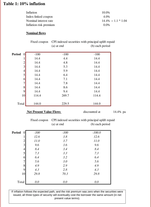
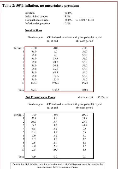
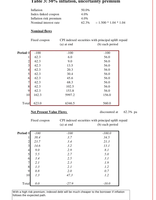
The payment stream of indexed bonds is typically back-loaded. Normally that part of the yield which relates to actual inflation is effectively capitalised and repaid on maturity (if the principal is indexed and all principal is repaid on maturity rather than during the life of the security). This reduces the government’s budget deficit on a cash basis in the early years of a bond’s life. An irresponsible government might be tempted to loosen fiscal policy accordingly, leaving the burden to be borne by later governments/generations. If the market perceived this to be case, the government’s anti-inflation credibility would be weakened. (The same argument would hold for the issuance of zero coupon securities with a maturity of more than one year.)
The tables in Appendix 2 indicate the cash flow profiles of fixed coupon and indexed securities, with two variations on indexation. In the first, the inflation payment is all made at redemption, so that the cashflow is low during the life of the security and high at the end20. This may suit the demands of some investors well - particularly in a relatively high inflation economy - and so reduce the cost of finance21. The second pays the inflation uplift at the end of each coupon period. This means that, ex ante, the payments flow will be similar to that for a fixed coupon security - assuming that no ‘inflation premium’ is paid on the latter and that the level of inflation is expected to be stable. Ex post, the pattern and sum of payments will be different, to the extent that the inflation outturn differs from expectations. The columns at the bottom of each table show the net present value of the cash flows, using the nominal yield on the fixed coupon security as a deflator. [A third possible payments flow - zero
20
The duration (the weighted average term to maturity of the discounted cash flows) of such
securities will be higher than for fixed interest securities with the same maturity. (See Section 5.1 for further discussion of duration).
21 A discussion of investor preference and potential benefits to the government as issuer in identifying the “preferred
coupon, where the real interest as well as the inflation uplift are paid on maturity, is not illustrated here. This method has been used in Iceland, Poland and Sweden.]
Figures for each type of security are shown for two different expected inflation rates: 10% and 50%; and there is a variant for the 50% inflation rate scenario, with an inflation risk premium payable on the fixed coupon security. It is clear from the tables that the cash flows for the different types of security diverge increasingly as inflation rises.
4.5 Convertible bonds
Some governments have issued convertible bonds. These normally offer the investor the option of converting from one type of security to another, e.g. short to long-term or vice versa, fixed to floating or indexed. In issuing them the government hopes that the investor will pay a premium for the option, and that this premium will more than offset the cost to the government if the option is exercised.
Equity-convertible bonds may be useful if the government is planning to privatise certain assets, such as state-owned enterprises, and wishes to obtain some of the value of the privatisation proceeds early. For instance, a security convertible into an equity could be sold for 100, redeemable in 2 years time or convertible at the investor’s option into, say, 10 shares of a certain enterprise which is to be privatised. If the estimated market value of that enterprise rises during the period, the investor will exercise his option and convert; and if its value has risen much faster than expected, the opportunity cost to the government - through selling the option to buy at a fixed price - may outweigh the premium received for selling the option. If the enterprise’s estimated value falls, the investor will buy the shares more cheaply in the market and not exercise the option. If it turns out, for whatever reason, that the enterprise is not privatised, some compensation may need to be paid to the investor.
4.6 Zero coupon bonds and strips
A zero coupon bond has only one (redemption) payment and is sold at a discount to its face value. In pricing the bond, it will be discounted at its spot rate i.e. the rate of discount specific to that maturity.
The price of a zero coupon bond is therefore given
by:-Price =
) 1
( Zi
R
+
Where R is the redemption payment
The discount rate used (Zi ) can be thought as the redemption yield of a zero-coupon bond.
The zero coupon bond has a number of advantages over its conventional counterpart. The zero coupon bond consists of a single point cash flow and therefore, by purchasing a selection of such bonds, the investor can build up the cash flows he wants, rather than receiving - and possibly needing to reinvest - frequent coupons. This allows far more efficient asset/liability management and eliminates reinvestment risk. Zero coupon bonds can therefore be used as building blocks from which to construct financial instruments such as annuities or deferred payment bonds.
A zero coupon bond also has greater duration (for the same maturity) and greater convexity (for the same duration) than coupon bonds. (See Section 5 for a more detailed discussion on duration and convexity.) This makes them potentially attractive to a large part of the market; for example, traders, who trade on risk and are looking for increased volatility; investors who want long duration assets; fund managers who are seeking to match the duration of their portfolios and have, for example, long duration pension liabilities.
Before issuing zero coupon bonds, governments will wish to know where on the yield curve the demand is. This is usually at the short end (as traders are keen to trade these potentially volatile instruments) or at the long end where duration is high. Because there is less obvious demand for the medium maturity zeroes, some players may be less willing to strip a bond (see below) for fear of having these relatively high duration products sitting on their balance sheets. For this reason, central banks may be willing to take them as collateral in their monetary operations in order to give some utility.
Depending on government accounting methods, some governments may be a little averse to zero coupon issuance as the monies received at issuance will obviously be less than a coupon bond of the same maturity.
Strips
A strip is a zero coupon bond, derived from separating a standard coupon-bearing bond into its constituent interest and principal payments that can then be separately held or traded as zero-coupon bonds22. For example, a 5-year bond with an annual coupon could be separated into six zero-coupon bonds, five representing the cash flows arising from coupons and one relating to the principal repayment. For £100 nominal worth of this bond with, say, a 6% coupon paying on 1 June each year the following cashflow would result from
22
Chart 4.6
Thus, stripping would leave five zero coupon bonds of £6.00 (nominal), maturing on 1 June each year and one zero coupon bond of £100 (nominal) maturing on 1 June in five years time.
As most strip markets trade on yield rather than price, it follows that a standard yield formula should be used to calculate settlement value, to avoid any disputes. The Bank of England designated the following price/yield relationship for the UK government securities strips market:
n sr
2
y
1
100
P
+
ö
ç
è
æ
+
=
where: P = Price per £100 nominal of the strip
y = Gross redemption yield (decimal) ie if the yield is 8% then y = 0.08
r = Exact number of days from the settlement/issue date to the next quasi-coupon date
s = Exact number of days in the quasi-coupon period in which the settlement date falls
0 20 40 60 80 100 120
Time
and: - r&s are not adjusted for non-working days
- The Bank of England proposed that yields be quoted to 3 decimal places and prices quoted to a maximum of 6 decimal places
- A quasi-coupon date is a date on which a coupon would be due were the bond coupon bearing rather than a strip.
- The formula is the semi-annual equivalent of the French Tresor formula and it differs from the US formula in using compound rather than simple interest for the shortest strip.
- The yield is divided by 2 because the UK government strips market is based on and deliberately quoted to be compatible with the underlying market, in which bonds are quoted on a semi-annual basis.
If investors see stripping as a useful process, then they should be willing to pay a premium for the product, thereby reducing yields on strippable stocks (and therefore lowering funding costs). However, there are costs to setting up a stripping operation and the authorities will need to know whether investors would find it useful before embarking on this exercise.
In this respect, there are a number of issues to consider before setting up a strips market. Some of the most important are set out
below:-• It is important to make the strips market as (potentially) liquid as possible. If all stocks are strippable, but all have different coupon dates, then the strips derived from each coupon will be relatively small. However, if stocks have the same coupon date, and the coupon strips from different stocks are fungible, this will obviously make for a more liquid market. In this case, once a stock is stripped each coupon strip is simply a cash flow with a particular maturity date: the original parent stock is no longer relevant. (A Bank of England paper ‘The Official Gilt Strips Facility: October 1997’ published shortly ahead of the start of the UK strips market, provided details of the cash flows on strippable stocks, demonstrating the potential strips outstanding.)
• The stripping and reconstitution process must be straightforward and relatively inexpensive in order to encourage market players to strip the stock.
• All profit on a strip is capital gain and therefore any anomolies between capital gains tax and income tax should be reduced or, ideally, removed before introducing stripping. It is important that there are no tax advantages to stripping, otherwise the market will trade on anomolies rather than fundamentals. It could also mean that any gain from lower funding costs is more than offset by the reduced tax income.
Further details on the issues facing the UK strips market before its introduction can be found in ‘The Official Gilt Strips Facility’: a paper by the Bank of England’: October 1997. Having introduced a strips market in the UK in December 1997, by the end June 2000, just over £2.8 billion (2.2%) of strippable gilts were held in stripped form and weekly turnover in gilt strips averaged around £50 million nominal, compared with around £30 billion nominal turnover in non strips.
5 Measures of risk and return 5.1 Duration
In the past, there were various ways of measuring the ‘riskiness’ of the bond, and perhaps the most common was the time to maturity. All other things being equal, the longer the bond the greater the volatility of its price (risk). However, this measure only takes into account the final payment (not any other cash flows), does not take into account the time value of money and therefore does not give an accurate comparison of relative ‘riskiness’ across bonds. For example, is an eleven-year bond with a 10% coupon more risky than a ten-year bond with a 2% coupon?
Duration is a more sophisticated measure as it takes into account all cash flows and the time value of money. ‘Macauley duration’ measures, in years, the riskiness (or volatility) of a bond by calculating the point at which 50% of the cash flows (on a net present value basis) have been returned. Duration is therefore the weighted average of the net present values of the cash flows. It allows us to compare the riskiness of bonds with different maturities, coupons etc. In calculating the net present values of the cash flows, it is Redemption Yield that is used as the discount rate.
In mathematical terms, this is expressed
as:-Macauley Duration =
P t CF PV t
n ×
=
Where PV CF( t)= Present value of cash flow at time t t = time (years) to each particular cash flow P = price of the bond (dirty)
It is perhaps easier to look at this pictorally. For a 5-year bond with a 10% annual coupon, imagine that the shaded area represents the net present value of each cash flow; and that the shaded areas are weights along a seesaw. The Macauley duration is the point at which the seesaw balances.
Chart 5.1
The relation between Macauley duration, price and yield is given by
fc y 1
DxP
+ − = ∆ ∆
y P
(1)
Where ∆P/∆y = Proportional change in price with respect to change in yield P = price
y/fc = yield/frequency of coupon payments per annum D = Macauley duration
From Macauley duration, we can express Modified Duration, which is a measure of the price sensitivity of a bond:
Modified Duration = Macauley duration (1+ y
fc)
Time
Pa
y
m
en
ts
(
£
)
{
{
C
o
u
p
o
n
Pr
in
ci
pal
Net present value
C
oup
Substituting Modified Duration into equation (1) above, and slightly rearranging
gives:-= ∆ ∆
p y
P 1
Modified Duration (2)
Modified Duration describes the sensitivity of a price of a bond to small changes in its yield – and is often referred to as the volatility of the bond. It captures, in a single number, how a bond’s maturity and coupon affect its exposure to interest rate risk. It provides a measure of percentage price volatility, not absolute price volatility and is a measure of the percentage price volatility of the full (i.e. dirty) price. For any small change in yield, the resulting percentage change in price can be found by multiplying yield change by Modified Duration as shown
below:-% change in price = - (Modified Duration) x yield change (in basis points) (3)
The negative sign in the equation is, of course, necessary as price moves in the opposite direction to yield.
Factors affecting duration
Other things being equal, duration will be greater: the longer the maturity; the lower the coupon; the lower the yield. This is explained further below:
(i) Maturity
Looking at Chart 5.1, as maturity increases, the pivotal point needed to balance the seesaw will need to shift to the right and therefore duration will increase.
However, this shift to the right will not continue indefinitely as maturity increases. For a standard bond, duration is not infinite and the duration on e.g. a 30-year bond and a perpetual will be similar. This can be understood by looking again at the mathematics: the net present value of cashflows 30 years away are small, and the longer out, will get smaller. So, in calculating the duration, these terms (on the numerator) will become negligible. The maximum duration for a standard bond depends on the yield environment: for example, as at June 2000 the 30-year bond in the US had market duration of approximately 14 years; the longest duration Japanese bond was 18 years. The following diagram shows the approximate relationship between duration and maturity of the bond23:
y P
P =− ×∆
Chart 5.1b
The duration of a perpetual is given by
r r 1
D= +
For a zero coupon, (Macauley) duration will always equal the maturity. This can be seen from the formula as the zero coupon bond has only one cash flow and the price will be its present value. It is also obvious from Chart 5.1 as there is only one cash flow and the pivotal point will therefore be on the cash flow.
(ii) Coupon
Again, looking at Chart 5.1, we can see that as coupon decreases the pivotal point will again need to move to the right (an increase in duration) in order to balance the seesaw.
(iii) Yield
The relationship between duration and yield is perhaps less obvious from the above diagram but can be understood intuitively. As yields increase, all of the net present values of the future cash flows decline as their discount factors increase, but the cash flows that are farthest away will show the largest proportional decrease. So the early cash flows will have a greater weight relative to later cash flows and, on the diagram, the balancing point would need to move to the left to keep the seesaw balanced. As yields decline, the opposite will occur.
Portfolio duration
One use of duration is immunisation, where a portfolio of assets is selected such that its duration equals the duration of the liability portfolio. Many fund managers attempt to duration match their portfolios: this is more efficient than “duration matching” individual assets and liabilities. The duration of a portfolio is the weighted average duration of all the bonds in the portfolio i.e. the duration of each bond weighted by its
Years to maturity
11- 9 8 7 6 5 4 3 2
1-0 10 20 30 40
13-
12-Duration (years)
15-percentage within the portfolio (the 15-percentage within the portfolio is determined using present values).
The examples below show how bonds of different duration will be affected by changes in the yield curve.
Example 10
Consider a bond with Modified Duration of 9. Its yield increases by 10 basis points. The approximate percentage change in price is found by using equation
(2):-% change in price = -9(0.10) = 0.90
i.e. a fall in price of 0.9%
Example 11
Two ten-year bonds have durations of 6 and 8.5. There is a small shift in the yield curve such that both bond yields fall by 3 basis points. Calculate the percentage price change.
Bond 1
% change in price = -6(-.03) = +.18%
Bond 2
% change in price = -8.5(-.03) = +.255%
The bond with the higher duration will outperform.
If the bonds were trading at 96.30 and 98.20, the actual price rises would
be:-Bond 1
96.47 = price New 17 . 0 30 . 96 100
0.18× =
Bond 2
98.45 = price New 0.25 = 98.20 100
255 .
Example 12
The Modified Duration of a 10-year strip, currently selling at £85.50 (per £100 nominal), is calculated as
follows:-Macauley duration =
5 . 85
10 50 .
85 ×
= 10 years
Modified duration = 10
1+y (The yield can be calculated using the formula given in section 4.6 on page 33).
Limitations to using Modified Duration
However, there are limitations in using Modified Duration in predicting the price/yield relationship. It is only valid for small changes in yield; for parallel shifts in the yield curve; and for small time horizons. The reasons for these limitations can be more clearly seen from the graph below. The price/yield relationship estimated from the Modified Duration of a bond is linear (shown by the tangent to the curve at Po) whilst the actual price/yield relationship is a curve. There is therefore an error when using Modified Duration to estimate price movements.
Chart 5.1c
The graph shows that the larger the change in yield, the greater the degree of error in the price change calculated using modified duration. This error is primarily accounted for by convexity.
Error in estimating price change for a change in yield, using modified duration
Price/yield relationship from modified duration Actual
relationship
Price
Yield
5.2 Convexity
Modified Duration indicates how the price of a bond varies for small changes in yield. However, for large changes in yield, two bonds that have the same yield and the same Modified Duration can behave quite differently. This is due to the ‘error’ in using modified duration, as discussed above. This error is explained by convexity, which is the second derivative of a bond’s price with respect to yield. The convexity of a bond is a measure of the curvature of its price/yield relationship. Used in conjunction with Modified Duration, convexity provides a more accurate approximation of the percentage price change, resulting from a specified change, in a bond’s yield, than using modified duration alone24.
The approximate percentage price change due to convexity
is:-% price change = ½ x convexity x (percentage yield change)²
The convexity of a bond is positively related to the dispersion of the cash flows. Thus, other things being equal, if the bond’s cash flows are more spread out in time than another then it will have a higher dispersion and hence a higher convexity. Convexity is also positively related to duration.
Convexity is generally thought of as desirable and traders may give up yield to have convexity. This is because, in general, a more convex bond will outperform in an environment of falling yields, and will underperform less as yields rise. Furthermore, the convexity effect is asymmetric; for a specified fall in yields, the price rise on account of convexity will be greater (in magnitude) than the price fall related to the convexity factor for the same rise in yields. Convexity can therefore be associated with a bond’s potential to outperform. However, convexity is a good thing if the yield change is sufficient that the greater convexity leads to outperformance. (For only small changes in yield, the price change estimated by modified duration gives a good guide and therefore paying for convexity may not be worth it.) If convex bonds are overpriced in an environment of low volatility, some investors will want to sell convexity. And, of course, yields can shift suddenly leading to changes in convexity.