Ann. Geophys., 24, 2583–2598, 2006 www.ann-geophys.net/24/2583/2006/ © European Geosciences Union 2006
Annales
Geophysicae
Simulating radial diffusion of energetic (MeV) electrons through a
model of fluctuating electric and magnetic fields
T. Sarris1,2, X. Li1, and M. Temerin3
1Lab. for Atmospheric and Space Physics, Univ. of Colorado, Boulder, CO, USA 2Demokritus University of Thrace, Xanthi, Greece
3Space Sciences Lab, University of California, Berkeley, CA, USA
Received: 29 March 2006 – Revised: 4 July 2006 – Accepted: 19 July 2006 – Published: 20 October 2006
Abstract. In the present work, a test particle simulation is performed in a model of analytic Ultra Low Frequency, ULF, perturbations in the electric and magnetic fields of the Earth’s magnetosphere. The goal of this work is to ex-amine if the radial transport of energetic particles in quiet-time ULF magnetospheric perturbations of various azimuthal mode numbers can be described as a diffusive process and be approximated by theoretically derived radial diffusion coeffi-cients. In the model realistic compressional electromagnetic field perturbations are constructed by a superposition of a large number of propagating electric and consistent magnetic pulses. The diffusion rates of the electrons under the effect of the fluctuating fields are calculated numerically through the test-particle simulation as a function of the radial coor-dinateLin a dipolar magnetosphere; these calculations are then compared to the symmetric, electromagnetic radial dif-fusion coefficients for compressional, poloidal perturbations in the Earth’s magnetosphere. In the model the amplitude of the perturbation fields can be adjusted to represent realis-tic states of magnetospheric activity. Similarly, the azimuthal modulation of the fields can be adjusted to represent different azimuthal modes of fluctuations and the contribution to radial diffusion from each mode can be quantified. Two simulations of quiet-time magnetospheric variability are performed: in the first simulation, diffusion due to poloidal perturbations of mode numberm=1 is calculated; in the second, the diffusion rates from multiple-mode (m=0 tom=8) perturbations are calculated. The numerical calculations of the diffusion co-efficients derived from the particle orbits are found to agree with the corresponding theoretical estimates of the diffusion coefficient within a factor of two.
Correspondence to: T. Sarris
Keywords. Magnetospheric physics (Energetic particles, trapped) – Space plasma physics (Charged paricle motion and acceleration; Numerical simulation studies)
1 Introduction
Determining the source and acceleration mechanism of en-ergetic (MeV) particles is one of the main current subjects of research in radiation belt physics. It has been observed that often during periods of magnetic activity, combined with high solar wind velocity, electron acceleration occurs, evi-denced by MeV electron flux increases by a few orders of magnitude on time scales from hours to days (e.g. Paulikas and Blake, 1979; Baker et al., 1986). Many different ac-celeration and loss processes might occur during such times, acting on particles either adiabatically or non-adiabatically, depending on the time scale of each process. A review of the various transport and acceleration mechanisms that have been proposed to explain the orders-of-magnitude increase of particle fluxes is given in Li and Temerin (2001) and Fridel et al. (2002); a differentiation between the various mechanisms in terms of the changes they inflict on phase-space density is presented in Green and Kivelson (2004).
en-ergy. Such stochastic diffusion in the electrons’L-shell will result in a net increase or decrease on particle flux at a given location and energy, depending on the initial distribution of particles, and also on the existence of particle sources and losses in the magnetosphere. As Kivelson and Russel (1995) note, radial diffusion always has the effect of reducing the radial gradients of the distribution function at fixed first and second adiabatic invariants,µandJ. It remains to be seen if radial diffusion caused by ULF waves is capable of trans-porting enough plasma sheet particles into the inner magne-tosphere to explain the orders-of-magnitude increases in the fluxes that are often observed in the inner magnetosphere. It also remains open to quantify the contribution from various modes of ULF perturbations and to associate the contribution with the perturbations’ excitation mechanism.
Theoretical estimates of the diffusion rates of electrons, due to stochastic electric and magnetic perturbations, have been performed since the early years of radiation belt stud-ies (Falthammar, 1965; and later on, Schultz and Lanzerotti, 1974; Brizard and Chan, 2001). In these studies, the derived expressions for the diffusion rates are related to the spectral characteristics of broad-band magnetospheric random varia-tions. The diffusion rate of energetic electrons is described by the diffusion coefficient, DLL. The expression for the
diffusion coefficient of electrons in fluctuating fields was in-troduced by Falthammar (1965), who also made a distinction between electrostatic (DELL)and electromagnetic (DMLL) con-tributions to the total diffusion coefficientDLL, and derived
expressions forDLLE andDLLM as a function ofL. Electro-static diffusion is caused by perturbations in the convection electric fields, whereas electromagnetic diffusion is caused by perturbations in the Earth’s magnetic field and by the in-duced perturbating electric fields. The expressions forDELL andDLLM were also found to be dependent on the spectral power density of the fluctuating fields, and in particular, on the power spectral density at the particles’ drift frequency, since only fluctuations at frequencies close to the electrons’ drift frequencies can produce enhanced diffusion, through the drift-resonant interaction between ULF waves and the electrons. These derivations were non-relativistic and in-cluded contributions only fromm=1 mode, wheremis the azimuthal wave number (for a definition ofm, see below, Sect. 4.1.3). Recently, using a treatment similar to Faltham-mar (1965), Fei et al. (2006) derived theoretical calculations for the electric and magnetic diffusion coefficients of rela-tivistic electrons in a symmetric and an asymmetric magnetic field that included contributions from different modes.
Radial diffusion mechanisms have been used in various ef-forts to model radiation belt dynamics during different types of geomagnetic conditions. Modeling of outer zone electrons during a storm by Brautigam and Albert (2000) has indicated that additional heating by in-situ acceleration mechanisms was required to reproduce the observed electron fluxes of higherµ, while the flux enhancement of lowerµwas
ade-quately described by radial diffusion. A review of modeling efforts by Albert et al. (2001) concluded that radial diffu-sion provides an underlying and significant minimum level of transport that must be considered, and suggested that ex-isting radial diffusion formalism could be expanded to in-corporate other acceleration mechanisms. Radial diffusion calculations have also been performed using semi-empirical radial diffusion coefficients that successfully model and pre-dict MeV electron fluxes at geosynchronous orbit, based on solar wind measurements (Li et al., 2001; Li, 2004). Numeri-cal tests of radial diffusion in modeled field fluctuations have been performed in various studies: Elkington et al. (1999, 2003) investigated the interaction of particles in global, low-mtoroidal mode waves and found increased diffusion due to drift-resonance interactions; they associated the efficiency of radial diffusion processes to various characteristics of the magnetospheric variations, such as power spectral density, the presence of non-axisymmetric magnetic field, superim-posed toroidal oscillations, and strong convection electric fields. Perry et al. (2005) investigated the effects of magnetic and electric fields associated with poloidal mode ULF waves in a three-dimensional guiding center test particle code from which theL, energy, and pitch angle dependence of the dif-fusion rates were analyzed. Results from a dipole magnetic field model were compared to a compressed dipole model in the equatorial plane, and diffusion rates were shown to de-pend more strongly onLthan assumed in previous studies, particularly in times of intense ULF activity. Ukhorskiy et al. (2005) traced particles in narrow-band ULF waves with amplitudes similar to those often observed at CRRES, and found the diffusion rates due to toroidal waves to be very low; they also found that poloidal mode waves provide a much more efficient form of radial diffusion and therefore can play an important role in the dynamics of the outer ra-diation belt. Fei et al. (2006) used power spectral densities calculated from the MHD waves, produced by a global MHD simulation of a magnetic storm; test particles were traced in the global MHD fields, and their study showed that the radial diffusion coefficients describe the electron transport quite well, with the asymmetric terms making significant contri-butions at largerL-shells.
post-T. Sarris et al.: Simulating radial diffusion of energetic (MeV) electrons 2585 midnight region (Walker et al., 2005, pp. 233–244, and
ref-erences therein). These oscillations can be described as co-herent global oscillations of a magnetosphericL-shell with perturbations in the azimuthal directions. Poloidal oscilla-tions, on the other hand, take place in the magnetic merid-ian (e.g. Anderson et al., 1990), i.e. the poloidal direction; they are characterized by z-direction (perpendicular to the equatorial plane) or radial direction magnetic field pertur-bations and azimuthal electric field perturpertur-bations. Poloidal oscillations are also referred to as compressional and fast mode waves; they can be caused by either external pertur-bations at or beyond the magnetopause, or by internal ion anisotropies within the magnetosphere. In one description, poloidal oscillations can be excited by solar wind impulses incident upon the magnetospheric cavity; these waves can re-flect and become standing between an outer boundary (pos-sibly the magnetopause) and a turning point within the mag-netosphere (e.g. Mann and Wright, 1995). Poloidal oscil-lations could also be a consequence of mirror instability (e.g. Walker et al., 2005, pp. 233–244). It has been demon-strated by theoretical calculations and computer simulations that poloidal waves can be mode-converted to toroidal waves which are resonantly excited on closed magnetic field lines where the frequency of the poloidal waves matches the local Alfv´en frequency (Kivelson and Southwood, 1985; Wright and Rickard, 1995). In the process they transfer their pertur-bation energy and are thus dampened.
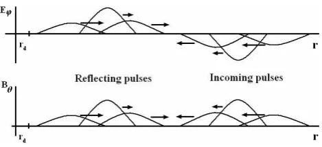
In this paper we present a model of random field fluctua-tions that aims in reproducing poloidal, compressional per-turbations of various modes. In this model, random field fluctuations are created by a superposition of earthward prop-agating Gaussian electric and consistent magnetic pulses that are reflected 100% at an inner limit. They are superimposed on a symmetric background magnetic field. The superposi-tion of the randomly initialized pulses produces a broadband fluctuation in the magnetic and electric fields that mimics well the observed spectral characteristics at geosynchronous orbit. The magnetic field pulses have a northward component and the consistent electric field has an azimuthal component; thus, based on the results from previous research and also based on the observational characteristics that are described in the next section, we assume in the following that the field perturbations represent poloidal, compressional, fast-mode (also called storm-time) ULF pulsations.
Energetic electrons are traced under the effect of the mod-eled fluctuating fields, and the diffusion rates of the electrons are calculated numerically. In this study we focus on en-ergetic electrons in the energy range from hundreds of keV to a few MeV. We are particularly interested in electrons of these energies since they are often of significant flux to cause spacecraft malfunctions and pose threats to astronauts in the inner magnetosphere (e.g. Gussenhoven et al., 1991; Baker et al., 1998a, 1994). The frequency range of ULF pertur-bations that is close to the drift frequency of these electrons is 1.5 to 10 mHz, and has been termed the Pc-5 range (see
Figure 1. The field fluctuations are produced in the model by the superposition of a large number of electromagnetic Gaussian pulses that propagate earthward and are reflected 100% at an inner boundary rd.
33
Fig. 1. The field fluctuations are produced in the model by the su-perposition of a large number of electromagnetic Gaussian pulses that propagate earthward and are reflected 100% at an inner bound-ary rd.
classification by Jacobs et al., 1964).
Two different azimuthal localizations of poloidal compres-sional pulsations are simulated: pulsations that extend across the whole dayside magnetosphere and have a null at mid-night, and pulsations extending across a fraction of the day-side region. The two simulations of different azimuthal ex-tents are compared to the azimuthal modes of compressional fluctuations; the first case simulates fluctuations with contri-butions from the primary, global-oscillation mode (m=0) and first mode (m=1), whereas the second case simulates a lo-calized fluctuation with contribution from modes, with mode numbersm=0 tom=8. In the simulated fluctuations we trace relativistic electrons of single-µ values. Through their ra-dial displacement in time, we calculate the diffusion rates of the electrons for the two cases. The diffusion rates obtained through the simulation are compared to existing theoretical calculations, which associate the diffusion rate of the elec-trons with the Power Spectral Density, PSD, of the fluctua-tions.
2 Observations
The model presented in this work simulates compressional Pc-5 fluctuations in the magnetosphere. Some of the reported characteristics of compressional fluctuations, as derived from observations and modeling, are the following:
1. Compressional Pc-5 pulsations, as well as toroidal and poloidal mode field line resonances appear to account for most of the observed pulsations in the outer magne-tosphere (Anderson et al., 1990). In their study, Ander-son et al. recorded pulsations as compressional when the dominant spectral feature appeared in the radial and northward components.
[image:3.595.311.546.61.168.2]sources are the solar wind (Barnes, 1983), the foreshock (Greenstadt et al., 1980), the bow shock (Greenstadt et al., 1979; Takahashi et al., 1981) and the magnetopause (Kepko et al., 2002).
3. Storm-time compressional pulsations are localized in latitude, occurring within 15◦of the magnetic equator. Storm-time Pc-5 type waves display a systematic varia-tion in latitude distribuvaria-tion withL, being more localized near the equator for lowLthan for highL(Anderson et al., 1990).
4. Compressional pulsations have been observed between 8 and 12 RE near dusk with HEOS 1 (Hedgecock,
1976), suggesting that a significant number of these waves occur at distances greater than 6.6RE.
5. The power of compressional pulsations in the Pc-5 fre-quency range is enhanced characteristically during the main phase of magnetic storms (Baker et al., 1998b; O’Brien et al., 2001), establishing the link between the solar wind and magnetospheric Pc-5 fluctuations. 6. The propagation of a disturbance in the magnetosphere
has been modeled several decades ago (e.g. Francis et al., 1959; Nishida, 1964; Burlaga & Ogilvie, 1969). In some descriptions, solar wind impulses incident upon the magnetospheric cavity can excite inward traveling compressional impulses which propagate with the speed of a fast mode, magnetosonic wave.
7. Compressional waves propagating within the magneto-spheric cavity can reflect and become standing between the magnetopause and a turning point within the mag-netosphere (Mann and Wright, 1995), which could be the plasmapause.
8. As compressional impulses propagate into the magne-tosphere across magnetic shells, they continuously pro-duce transverse waves via mode conversion due to the inhomogeneity of the propagation media (ring-current and plasmaspheric plasma) and also because of the curved geometry (Hasegawa et al., 1983; Mann and Wright, 1995). Thus, polarization and amplitude, as well as arrival times based on any local measurements are expected to strongly depend on wave coupling and dipolar geometry in the magnetosphere (Lee & Lysak, 1999).
3 Model Description
The model that has been used in this work reproduces com-pressional electromagnetic field fluctuations by a superposi-tion of a large number of propagating Gaussian pulses. In this section we first describe the formulation of a single pulse; we then present the process of randomization and superposition
of a large number of such pulses, and finally, we compare the produced model field signatures with real measurements at geosynchronous orbit.
3.1 Single pulse
In the spherical coordinate system(r, θ, φ)the electric field of a single pulse is given by the following equation:
Eφ= − ˆeφE0(1+cos(φ−φ0))p
exp(−ξ2)−exp(−η2)
, (1)
where ξ=(r−ri+v0t )/d determines the location of the maximum value of the incoming pulse and η=(r−2ri+rd−v0t )/d determines the location of the reflecting pulse; rd determines the location where the
reflection occurs;dis the radial width of the pulse;v0is the radial speed of the pulse;eˆφis the azimuthal direction;E0is the electric field amplitude;p (=1 and 8 in the simulations presented) describes the local time dependence of the electric field amplitude, which is largest atφ0; and ri is a
parameter in the simulation that determines the arrival time of the pulse. From Eq. (1) the pulse electric field is positive, or westward, for incoming pulses and negative, or eastward, for reflecting pulses, as indicated by the minus sign of the second term in the brackets. The consistent magnetic field of the propagating electric pulse of Eq. (1) is obtained from Faraday’s law, after performing the curl calculation of Eq. (1) in spherical coordinates and integrating:
Bϑ= − ˆeϑ
E
0
v0
(1+cos(φ−φ0))p
exp(−ξ2)+exp(−η2)+
d√π 2r
(erf (ξ )+erf (η))
(2) whereerf (x)=2/√
π ∞
R
0
e−x2dxis the error function. Each magnetic pulse is superimposed on a background magnetic field, BE, which is time-independent and is
con-sidered a simple dipole field in the present simulation. The pulse field and background field satisfy Eφ·(Bθ+BE)=0
and∇ ·(Bθ+BE)=0. In the simulation we consider only
equatorially mirroring electrons, which move on average ac-cording to the relativistic guiding center equation described in (Northrop, 1963):
υd=c
Eφ×B
B2 + µc γ q
B× ∇⊥B
B2 , (3)
wherecis the speed of light in vacuum,γ is the relativistic correction factor:γ = 1−v2/c2−1/2
,µis the relativistic adiabatic invariant (see Sect. 4.1.1), Eφis the vector electric
T. Sarris et al.: Simulating radial diffusion of energetic (MeV) electrons 2587 3.2 Multiple pulses
A large number (1200) of random pulses, such as those de-scribed in Sect. 3.1, were superimposed; a schematic of the superposition and propagation of the pulses is given in Fig. 1. Each pulse was initiated with a random amplitudeE0in the range from 0.005 mV/m to 0.015 mV/m, a random pulse ve-locityv0in the range from 300 km/s to 500 km/s and a ran-dom distanceri in the range from 2·108m to 6·108m, where
riis a parameter that determines the arrival time of the pulse
in the simulation. The radial width of the pulses was kept constant at the valued=4·108m. Angle φ0 was set to 0◦, meaning that all the pulses have a maximum at noon and a null at midnight. A random number generator was used in determining the pulse parameters. One hundred different runs were performed for different random number generator initialization integers (“seeds”) and the individual field spec-tral calculations (see Sect. 4.1.4) as well as the calculations for the electron average squared displacements (see Sect. 4.2) were averaged together.
3.3 Comparison of model fields to data
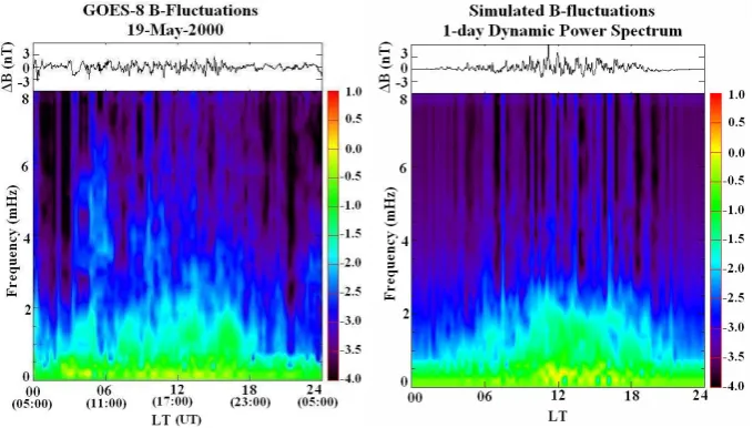
In order to check the validity of the simulation, the model magnetic field was compared against the magnetic field sig-nature at geosynchronous orbit, as measured by GOES-8 on an average (in terms of magnetospheric activity) day. One-minute GOES-8 measurements were used; for this sampling frequency, the Nyquist frequency (and hence the maximum frequency we can monitor in this data set) is 8.3 mHz. To per-form the comparison, the Dynamic Power Spectra of the sig-nal time series were calculated, in order to visualize the local time dependence of the ULF fluctuations. This was done by sliding a Hanning window through the data and performing an FFT on the subset of the signal within the window. A 1-day signal includes 1440 data points under a 1-min sampling time; the FFT length of the window was 83 points and there were 79 overlapping FFT blocks in one day’s signal in the analysis performed. The frequency resolution in this analy-sis was 0.2 mHz. An example of the Dynamic Power Spectral Density of one day’s GOES-8 data is shown in the left panel of Fig. 2. In this figure, the field variation in the ULF regime is plotted in the top panel, and the power spectral density in the lower panel. The field variation is calculated by subtract-ing the large-scale variation (e.g. diurnal variation and other large-scale changes) from the original signal; the large-scale variation is calculated using a wavelet signal decomposition scheme, with a Daubauchies wavelet and 25 coefficients (for a review see, e.g. Rioul, 1991). In this day, most of the fluctuations are in the z-direction (indicating compressional fluctuations); it is also a day with a smooth diurnal variation, without any indications of multiple processes going on at the same time.
In order to place the magnetospheric fluctuations of the selected day shown in the left panel of Fig. 2 in the context
of the average behaviour of the magnetosphere, a survey of the average Dynamic Power Spectra of ULF magnetic field fluctuations has been conducted, using 8 years of geosyn-chronous magnetic field measurements from GOES-8 satel-lite. In this survey, daily calculations of the Dynamic Power Spectra of the magnetic field, computed in exactly the same manner as described above, were averaged together. The av-eraging was performed for two cases: in one case the Dy-namic Power Spectra from all days were used; in the second case only the days with a daily mean|Dst|value of less than 20 were used. The study has shown that the selected day has ULF power that is one order of magnitude less than the aver-age power of all days of the 8 year survey; the ULF power of the selected day is of the same order of magnitude with the average power from all days, with a daily mean|Dst|value of less than 20.
The signatures produced by the model propagating pulses were recorded at geosynchronous orbit using the same sam-pling frequency as GOES-8 measurements, so that the model fluctuating fields could be compared to the data. The spacecraft’s motion around the Earth was also simulated. The modelled magnetic perturbation signal and its dynamic power spectrum are shown in the right panel of Fig. 2, keep-ing the same format as in the left panel. From the compari-son of the upper panels of the two figures we note that there is low-frequency fluctuation in the midnight region in the GOES-8 data, contrary to the model; however, these fluctua-tions are below the 1.5 to 10 mHz range of ULF fluctuafluctua-tions that are of interest in this study. In general, the model man-ages to reproduce in a realistic way the power contained in the Pc-5 fluctuations of the magnetic field at geosynchronous orbit for this particular day.
4 Radial Diffusion Coefficients
In this section the effect of the model field fluctuations on a set of energetic electrons of a singleµ-value is explored, as it is expressed by the diffusion coefficientDLL. The
ex-pressions for the magnetic diffusion coefficient are first de-scribed, as they were formulated by Falthammar (1965) and generalized by Fei et al. (2006), and the various terms in-volved are discussed. We then show the results from test-particle simulation in a background dipole magnetic field with superimposed field fluctuations, and we calculate nu-merically the diffusion coefficientDLL. Based on the model
characteristics and on the discussion in Falthammar (1965), we relate the simulated diffusion coefficient toDLLB,Sym, the symmetric magnetic diffusion coefficient.
Figure 2. Comparison of one day of GOES-8 magnetic field measurements with one day of simulated model magnetic field. On the upper left panel the diurnal large-scale variation has been subtracted from the data using wavelet decomposition, to reveal the fluctuation level in the ULF regime. On the lower panel, color-coded is the power of the magnetic field signal as a function of frequency and time (dynamic power spectrum); the units in the color scale correspond to the logarithm of the power, in nT2/Hz. The fluctuations and the spectra of the magnetic field are plotted in time for 24h from 0500UT, when GOES-8 is located at midnight, to 0500UT of the next day. On the right-hand side, the model magnetic field is recorded at geosynchronous orbit with the same time resolution and duration as the GOES-8 measurements. Spacecraft motion around the Earth is also simulated. An azimuthal amplitude modulation of: 1+cos(φ) was used in this simulation.
[image:6.595.129.469.58.251.2]34
Fig. 2. Comparison of one day of GOES-8 magnetic field measurements with one day of simulated model magnetic field. On the upper left panel the diurnal large-scale variation has been subtracted from the data using wavelet decomposition, to reveal the fluctuation level in the ULF regime. On the lower panel, color-coded is the power of the magnetic field signal as a function of frequency and time (dynamic power spectrum); the units in the color scale correspond to the logarithm of the power, in nT2/Hz. The fluctuations and the spectra of the magnetic field are plotted in time for 24 h from 05:00 UT, when GOES-8 is located at midnight, to 05:00 UT of the next day. On the right-hand side, the model magnetic field is recorded at geosynchronous orbit with the same time resolution and duration as the GOES-8 measurements. Spacecraft motion around the Earth is also simulated. An azimuthal amplitude modulation of: 1+cos(φ)was used in this simulation.
adiabatic invariants of the electrons (Schulz and Lanzerotti, 1974; Bourdarie et al., 1997). When the first two adiabatic invariants are conserved but the third one is violated, the re-sulting expression is the radial diffusion equation, expressed as:
∂F ∂t =L
2 ∂ ∂L
D
LL
L2 ∂F ∂L
, (4)
at constant first adiabatic invariantµ and second adiabatic invariantJ. In Eq. (4),F is the electron phase space density and is related to the more experimentally familiar quantityj, the electron differential flux, by: F=j/p2,wherep is the electron momentum. The radial diffusion coefficient,DLL,
is obtained by integrating the instantaneous rate of change of the shell parameterLfor a large number of particles, over an interaction timeτ >>2π/, whereis the particle drift frequency:
DLL≡
(1L)2
2τ . (5)
In the above expression, the brackets denote integration over timeτ, and 1 denotes an average over a large number of particles [see also Schultz and Lanzerotti, 1974, pp. 89–92]. The magnetic diffusion coefficient,DB,SymLL , produced by electromagnetic fluctuations on particles of a singleµ-value that are drifting in a symmetric background magnetic field, has first been derived theoretically by Falthammar (1965). This derivation is non-relativistic and includes only single-mode fluctuations of single-mode numberm=1. Recently, Fei et
al. (2006) generalized Falthammar’s expression to include relativistic electrons and multiple mode numbers of fluctu-ation. The expression they derived has the following form:
DB,SymLL = µ
2
8q2B2
ER4E
L4 γ2
! ∞ X
m=1
m2PmB(mωd). (6)
In the above equationµis the value of the first adiabatic in-variant of the electrons considered,q is the electron charge, γ is the Lorentz relativistic factor,BE is the magnetic field
strength at the surface of the Earth, RE is one Earth
ra-dius,mis the azimuthal mode number of the fluctuation and PmB(mωd)is the power spectral density of the compressional
wave magnetic field at frequencym-times the drift frequency ωdof the electrons considered. The summation is performed
fromm=1 to infinity for all participating modes. In the fol-lowing we comment on some of the terms in Eq. (6): the first adiabatic invariantµ, the Lorentz relativistic factor γ, the mode number of fluctuation m, and the power spectral densityPmB at frequency mωd.
4.1.1 First adiabatic invariant,µ
In Eq. (6), µ, the relativistic adiabatic invariant associ-ated with the electrons’ gyro-motion, can be written as: µ=p2⊥
2m0B, wherep⊥is the electron’s perpendicular
T. Sarris et al.: Simulating radial diffusion of energetic (MeV) electrons 2589
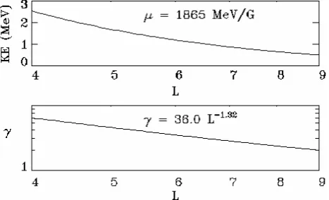
Figure 3. Upper panel: Kinetic energy of electrons as a function of L for a single first adiabatic invariant, μ= 1865 MeV/G. Lower panel: L-dependence of γ, the Lorentz relativistic correction factor, for μ= 1865 MeV/G.
.
35
Fig. 3. Upper panel: Kinetic energy of electrons as a function ofLfor a single first adiabatic invariant,µ=1865 MeV/G. Lower panel:L-dependence ofγ the Lorentz relativistic correction factor, forµ=1865 MeV/G.
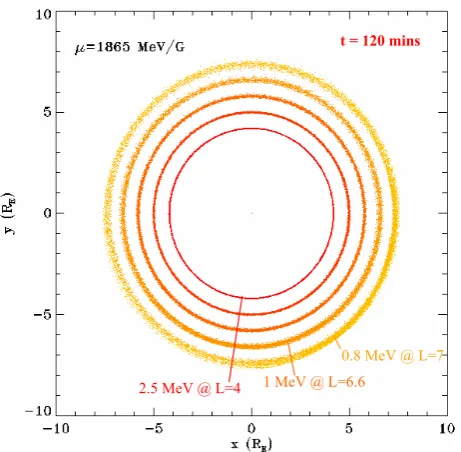
increasingL. The Kinetic Energy (KE) versusLrelation for theµ-value used in the simulation,µ=1865 MeV/G, is given in the upper panel of Fig. 3. Thisµ-value corresponds to electrons of energy 2.5 MeV atL=4.0, 1 MeV atL=6.6, and 0.7 MeV atL=8.0.
4.1.2 Lorentz relativistic factor,γ
The Lorentz relativistic correction factorγ can be expressed as:γ =(KE+m0c2)/m0c2, where KE is the electron’s kinetic energy, m0 is the electron rest mass and cis the speed of light. As mentioned above, for particles of a singleµ-value the kinetic energy decreases with increasing L. From the
KE-versus-Lrelation and from the expression forγ we can
calculate theγ-versus-L relation. For the electrons traced in the simulation, which have aµ-value of 1865 MeV/G, the L-dependence of the Lorentz factor is plotted in the lower panel of Fig. 3 and can be approximately fitted as: γ=36·
L−1.32. In the non-relativistic case,γ is equal to one at allL; in the ultra-relativistic limit,γ is proportional toL−1.5 and the factorL4/γ2in Eq. (6) is proportional toL7.
4.1.3 Mode number of compressional ULF fluctuations,m Theoretically, the fluctuating electric field of the Earth along the equatorial plane at any given time t could be approxi-mated by an expansion of a Fourier series of the form (simi-larly for the magnetic field):
E(t, φ)=12E0(t )+ ∞ P
m=1
am(t )·cos(mφ)+
∞ P
m=1
bm(t )·sin(mφ)
. (7)
In this expansion, m describes the mode of fluctuation of each component in the generalized Fourier series;αm(t )and
bm(t )are the time-dependent coefficients of the fluctuating
electric field, andE0(t) describes the global oscillations of the magnetosphere (global compressions and relaxations), corresponding to mode numberm=0. We note here that the
E E
φ φ
E E
t t
Figure 4. In the upper panels, the amplitude of the ULF perturbation electric field is given as a function of the azimuthal angle φ for idealized m=1 (left panel) and m=2 (right panel) poloidal modes of fluctuations. In the lower panels, the amplitude of the electric field that a particle experiences while drifting at a frequency ωD = mω is given as a function of time.
36
Fig. 4. In the upper panels, the amplitude of the ULF perturbation electric field is given as a function of the azimuthal angleφ for idealizedm=1 (left panel) andm=2 (right panel) poloidal modes of fluctuations. In the lower panels, the amplitude of the electric field that a particle experiences while drifting at a frequencyωD=mωis given as a function of time.
m=0 mode of global oscillations is not included in the sum of Eq. (6), since it does not contribute to particle radial dif-fusion: global fluctuations of the magnetic field will cause a fluctuation in the radial distance of a particle, however, the net radial displacement of the particle averaged over a time period much longer than the particle’s drift period will be zero, as long as there is no net increase or decrease in the global magnetic field intensity. In contrast, the non-zero modes of fluctuations can produce a net radial displacement to some particles, by what has been described as enhanced radial transport (diffusion) by drift resonance.
The concept that an energetic particle undergoing a peri-odic azimuthal drift at a particular drift frequencyωdaround
the Earth can experience a resonant acceleration, due to the interaction with electric field perturbations that do not aver-age to zero over the particle’s drift orbit, has been recognized early on in magnetospheric physics (Dungey, 1964). This resonant condition has been expressed as:
ω−mωd=0, (8)
where ω is the frequency of the field perturbations, ωd is
the drift frequency of the particle and m is the azimuthal mode number. The drift resonance of particles with fluctuat-ing fields is demonstrated in Fig. 4, which gives a schematic of the azimuthal and temporal characteristics of a fluctuating monochromatic electric field for two cases, corresponding to an idealized poloidalm=1 (left panels) andm=2 (right pan-els) mode of perturbation, respectively. In the left panels of Fig. 4, the perturbation is modulated by a cos(φ) function, whereas in the right panels the perturbation is modulated by a cos(2φ) function. In the upper panels of Fig. 4, the am-plitude of the electric fields is plotted versus the azimuthal angleφ for one time instancet0. The electric field in both plots points in the azimuthal direction, with eastward (west-ward) being positive (negative). The lower panels of Fig. 4 show the drift-resonant interaction of a particle drifting with a frequencyωdaround the Earth with an electric field
pertur-bation at the same frequency,ω=ωd, for anm=1 mode (left
panel), and twice the drift frequency, ω=2ωd, for an m=2
[image:7.595.311.545.60.138.2]Figure 5.Comparison of one day of GOES-8 magnetic field measurements with one day of simulated model magnetic field. The selected day has ULF fluctuation activity more localized around noon, compared to Fig. 2. The panel layout is similar to Fig. 2. On the right-hand side, the azimuthal amplitude modulation is governed by an (cos(φ) + 1)p azimuthal dependence,
with p=8, producing pulses that are more localized around noon.
[image:8.595.129.469.59.251.2]37
Fig. 5. Comparison of one day of GOES-8 magnetic field measurements with one day of simulated model magnetic field. The selected day has ULF fluctuation activity more localized around noon, compared to Fig. 2. The panel layout is similar to Fig. 2. On the right-hand side, the azimuthal amplitude modulation is governed by an (cos(φ)+ 1)pazimuthal dependence, withp=8, producing pulses that are more localized around noon.
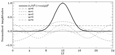
Figure 6.The azimuthal modulation of the earthward pulses by the factor (1+cos(φ))8 is given by the solid thick line, as a function of local time. The rest of the lines give the azimuthal modulation of the first five modes of fluctuation, as marked.
38
Fig. 6. The azimuthal modulation of the earthward pulses by the factor 1+ cos(φ)8is given by the solid thick line, as a function of local time. The rest of the lines give the azimuthal modulation of the first five modes of fluctuation, as marked.
the electron would experience along its drift path is non-zero for both cases, and hence the average workW˙=qE·V done by the electric field on the particle of speed V is also non zero.
In our model the amplitude of the fluctuating field fol-lows an azimuthal modulation of the form(1+cos(φ−φ0))p, which introduces a smooth transition from maximum fluc-tuations at noon (angleφ0)to zero fluctuations at midnight (angleφ0–π). The particular amplitude modulation was se-lected in order to match the spectral features that are com-monly observed in the radiation belts, which show enhanced fluctuations at noon. The exponentp determines the extent of the azimuthal dependence: a largep-exponent creates a modulation that confines the pulses aroundφ=0. Two sim-ulations are presented: in the first simulation an exponent of p=1 is used, which introduces an (1+cos(φ)) amplitude
modulation. The distribution of power of the model fluctua-tions in local time is given by the dynamic power spectra in the right panel of Fig. 2; in the same plot, the model fields are compared to measurements made on 19 May 2000 by GOES-8 spacecraft at geosynchronous orbit. A comparison with Eq. (6) shows that this amplitude modulation includes contributions from them=0 global mode and them=1 mode of ULF perturbations. As mentioned above, them=0 mode of global oscillations does not contribute to particle radial diffusion; hence we will refer to this simulation of field per-turbations as single-mode simulation.
In the second simulation performed, an exponentp=8 was used, modulating the azimuthal dependence of the fluctuat-ing fields as (1+cos(φ))8. This modulation creates a com-pressional perturbation that is azimuthally localized around noon. The distribution of power of the model fluctuations in local time is given by the dynamic power spectra of the right panel of Fig. 5. Such azimuthal localizations in the fluctu-ating fields are commonly observed: an example is given in the left panel of Fig. 5, which shows magnetic field measure-ments made by GOES-8 satellite on 5 February 1997. The format of the plot is similar to Fig. 2, with noon correspond-ing to the center of the plots and midnight to the edges of the plots. In order to determine which modes are included in the simulated perturbations of Fig. 5, and also in order to find the power at each mode, the azimuthal dependence fac-tor (1+cos(φ))8can be expanded as follows:
1 28
(1+cos(φ))8=0.2+0.35 cos(φ)+0.24 cos(2φ)
+0.13 cos(3φ)+0.06 cos(4φ)+ +0.017 cos(5φ)+0.0036 cos(6φ)
+0.0005 cos(7φ)+0.00003 cos(8φ)
[image:8.595.48.285.325.439.2]T. Sarris et al.: Simulating radial diffusion of energetic (MeV) electrons 2591
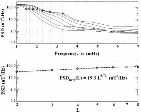
Figure 7(a).Top: The Power Spectral Density of the fluctuating fields in the single-mode simulation (m=1) is plotted with solid lines for various L from L=2 to L=8 as a function of frequency ω (in mHz). The highest line corresponds to L=2. The diamonds correspond to the power of fluctuations at frequency ωd (drift frequency of electrons of μ=1865 MeV/G) at the particular L. The power at these L is plotted in the lower panels as a function of L; a fit through these points gives the L-dependence function, PSDm=1(L).
Figure 7(b). The power of fluctuations for the multiple-mode simulation (m=1 to m=8) is plotted in a similar fashion. The diamonds correspond to fluctuations at frequency ωd; the asterisks correspond to fluctuations at frequency 2ωd.
39 Fig. 7. Top: The Power Spectral Density of the fluctuating fields
in the single-mode simulation(m=1) is plotted with solid lines for variousLfromL=2 toL=8 as a function of frequencyω(in mHz). The highest line corresponds toL=2. The diamonds correspond to the power of fluctuations at frequencyωd (drift frequency of elec-trons ofµ=1865 MeV/G) at the particularL. The power at theseL is plotted in the lower panels as a function ofL; a fit through these points gives theLdependence function, PSD(m=1(L)).
The constant term in the expansion represents anm=0 global mode of oscillation, which does not contribute to radial diffu-sion since it does not satisfy the resonance condition stated in Eq. (8). A comparison of Eq. (9) with Eq. (7) shows that there are nine modes of fluctuation in the model fields, with mode numbers fromm=0 tom=8. Figure 6 gives a graphical repre-sentation of the relative contribution of each term in Eq. (9). In this figure, the thick solid line marks the azimuthal depen-dence of factor (1+cos(φ))8, which modulates azimuthally all pulses in the simulation, producing a maximum at noon. The thinner lines give the azimuthal dependence of the various contributing modes of fluctuation as marked. The various terms are normalized, so that the sum of the amplitudes of all modes is one at noon.
It should be noted that, in the magnetospheric perturba-tions recorded on 19 May 2000 and 5 February 1997, mul-tiple modes of fluctuations of higher mode numbers might coexist at the same time, contributing to the total spectra in the left panels of Figs. 2 and 5; these cannot be distinguished from single-satellite measurements. However, in these par-ticular days, most of the magnetic field fluctuations were found in theBz (northward) component; we speculate that
they mostly correspond to quiet-time compressional fluctua-tions of the magnetopause, caused by solar wind variafluctua-tions, which are usually related to low-mmodes of fluctuations. Hence we find it reasonable to assume that most of the power contributing to radial diffusion in these days would be con-centrated in the lowest mode numbers of fluctuations.
Figure 7(a). Top: The Power Spectral Density of the fluctuating fields in the single-mode simulation (m=1) is plotted with solid lines for various L from L=2 to L=8 as a function of frequency ω (in mHz). The highest line corresponds to L=2. The diamonds correspond to the power of fluctuations at frequency ωd (drift frequency of electrons of μ=1865 MeV/G) at the particular L. The power at these L is plotted in the lower panels as a function of L; a fit through these points gives the L-dependence function, PSDm=1(L).
Figure 7(b). The power of fluctuations for the multiple-mode simulation (m=1 to m=8) is plotted in a similar fashion. The diamonds correspond to fluctuations at frequency ωd; the asterisks correspond to fluctuations at frequency 2ωd.
[image:9.595.311.544.62.248.2]39 Fig. 8. The power of fluctuations for the multiple-mode simulation
(m=1 tom=8) is plotted in a similar fashion. The diamonds cor-respond to fluctuations at frequencyωd; the asterisks correspond to fluctuations at frequency 2ωd.
4.1.4 Power spectral density of ULF electromagnetic per-turbations
The analytic expressions of the model fluctuating fields make possible the numeric calculation of the power of the fluctu-ations as a function of frequency and time at variousL; the calculations of the PSD that an electron drifting in a dipole field would experience at differentLare plotted in the up-per panels of Figs. 7 and 8 as solid lines, one for eachL, from L=2 to L=8. Fig. 7 corresponds to the single-mode simulation, whereas Fig. 8 corresponds to the multiple-mode simulation.
We are only interested in the power that will contribute to an electron’s radial transport, through the drift-resonant ef-fect of the ULF perturbations that was described above. The drift-resonant effect has been included in Eq. (6) of the diffu-sion coefficientDLLB,Symas contributions to radial diffusion only from fluctuations at frequencies mωd. Thus, the
to-tal PSD contributing to radial diffusion can be expressed for multiple modes of fluctuations as:
P SD= ∞
X
m=1
m2PmB(mωd), (10)
where PSD is measured inT2/Hz,mis the mode number of the ULF wave component andωdis the drift frequency of
[image:9.595.53.285.64.248.2]t = 120 mins
Figure 8. In the simulation particles of μ=1865 MeV/G were initialized in rings at various L. Particle locations are plotted after 2 hours of interaction with the fluctuating fields. Particle energy is color-coded, with inner particles (red) having highest energy.
1 MeV @ L=6.6
0.8 MeV @ L=7
2.5 MeV @ L=4
40 Fig. 9. In the simulation particles ofµ=1865 MeV/G were
initial-ized in rings at variousL. Particle locations are plotted after 2 h of interaction with the fluctuating fields. Particle energy is color-coded, with inner particles (red) having highest energy.
of Fig. 7 and 8 we plot vertical dotted lines at the drift fre-quenciesωdof electrons at variousL, fromL=2 toL=8, for
µ=1860 MeV/G. The power at each frequencyωd is marked
as a diamond. In Fig. 8, where the power of multiple-mode fluctuations is plotted, we also mark the power at frequencies 2ωd corresponding to mode numberm=2 with asterisks. In
the lower panels of Fig. 7 and 8 we plot the power at each frequencyωd as a function of theL-value corresponding to
that frequency, also with a diamond; similarly, we mark with asterisks the power at frequencies 2ωd. Thus, there is a
one-to-one relation between the asterisks and diamonds of the upper and lower panels of Figs. 7 and 8. We then perform a fit through the points in the lower panels of Figs. 7 and 8, and obtain the power-versus-L relationship for them=1 case in Fig. 7, and the m=1 andm=2 cases in Fig. 8. A simi-lar process is followed for the higher mode numbers for the multiple-mode simulation, which are not plotted here.
For the single-mode simulation the Power Spectral Den-sity as a function ofLis found to be:
PmB=1(ωd)=19.3·L0.71(nT2/H z) (11)
For the multiple-mode simulation, Table 1 gives an overview of the contribution to radial diffusion from the participating modes. The mode numbermis given in the first column; the relative power contribution from each mode,βm, is given in
the second column by the square of the normalized ampli-tude of each mode, which is the coefficient of each sine term in Eq. (9); and the relative contribution to the diffusion coef-ficient is given in the third column, by multiplyingβmbym2,
Table 1. The relative contribution of the participating modes to the diffusion coefficient.
m βm m2 βm PBm[nT2/Hz]
0 0.04 0.0 0
1 0.12 0.12 52*L1.11
2 0.06 0.23 11*L−0.03
3 0.017 0.15 10*L−0.44
4 0.0036 0.058 26*L−1.26
5 0.00029 0.0073 32*L−1.42
6 0.000013 0.00047 —
7 0.00000025 0.000012 —
8 0.0000000009 0.000000058 —
as indicated by Eq. (10). In the last column, the power spec-tral densityPmB is given as a function ofLfor each mode, calculated as described above. In Table 1, calculations ofPmB for them=6, 7 and 8 cases have been excluded, since they required calculation of the power of fluctuations at 6, 7 and 8 times the particles’ drift frequencies, respectively, which is well beyond the Pc-5 range of fluctuations that has been sim-ulated by the pulse model. However, the contribution of these modes to radial diffusion is insignificant, as is discussed be-low.
In order to calculate the theoretical diffusion coeffi-cient, by substitutingµ=1865MeV/G,γ=36·L−1.32,B0=0.31 Gauss andRE=0.6371×10⁷m, Eq. (6) can be written as:
DB,SymLL =5.77·106·L6.64·6m2PB(mωd). (12)
For the single-mode case, from Eqs. (12) and (11) we ob-tain:
DB,SymLL (m=1)=5.5·10−11·L7.35. (13)
For the multiple-mode simulation, from Eq. (12), using the expressions from the last column of Table 1 for the various PmBterms, we get:
DB,SymLL (m=1..8)=
1.8·L7.75+0.7·L6.61+0.4·L6.2
+0.4·L5.4+. . .·10−11. (14) 4.2 Numerical calculation of DB,SymLL from test-particle
simulation
[image:10.595.313.542.97.211.2]T. Sarris et al.: Simulating radial diffusion of energetic (MeV) electrons 2593
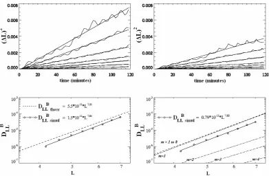
Figure 9. In the upper panels, each line represents the time evolution of the average squared
displacement,
(
Δ
L)
2, of particles evenly distributed in rings at various L from 4.6 (smallest
slope) to 7.0 (largest slope), every L=0.4. The fit to each line gives the rate of change of
<
(
Δ
L)
2> from which the radial diffusion coefficient at
L
is calculated. On the left (right)
panels, diffusion rates are calculated for the single-mode (multiple-mode) simulations. In the
lower panels, the radial diffusion coefficients at the various
L
are plotted as diamonds. The fit
through these points (solid line) gives the
L
-dependence of
D
LLB, in units of 1/sec. The
theoretical estimate for the diffusion coefficient is drawn with a dashed line both in the left
plot for the single-mode simulation, and in the right plot for the multiple-mode simulation. In
the multiple-mode simulation the contribution to the radial diffusion coefficient from the first
four modes is plotted with dashed-dotted lines.
41
Fig. 10. In the upper panels, each line represents the time evolution of the average squared displacement, (1L)2, of particles evenly distributed in rings at variousLfrom 4.6 (smallest slope) to 7.0 (largest slope), every L=0.4. The fit to each line gives the rate of change of<(1L)2> from which the radial diffusion coefficient atLis calculated. On the left (right) panels, diffusion rates are calculated for the single-mode (multiple-mode) simulations. In the lower panels, the radial diffusion coefficients at the variousLare plotted as diamonds. The fit through these points (solid line) gives theL-dependence ofDBLL, in units of 1/s. The theoretical estimate for the diffusion coefficient is drawn with a dashed line both in the left plot for the single-mode simulation, and in the right plot for the multiple-mode simulation. In the multiple-mode simulation the contribution to the radial diffusion coefficient from the first four modes is plotted with dashed-dotted lines.DB,SymLL as a function ofLwe initialize rings of electrons at variousL, fromL=4.6 toL=7.0 every dL=0.4, across all lo-cal times. We monitor the electrons under the effect of the fluctuating fields at each ring with a 2 min resolution. The positions of the rings’ electrons after 2 h simulated time are shown in Fig. 9. In this figure the electron energy is color-coded. It can be seen that there is anL-dependence of the diffusion rates, with electrons at largerLdiffusing more than electrons at lowerL. The diffusion coefficient at the particu-larLis then calculated from the slope of the average squared displacement, (1L)2, of a large number of electrons, as de-scribed by Eq. (5). In the upper panels of Fig. 10, the simu-lated (1L)2from electron tracing is plotted as a function of time for the selectedLvalues, together with the correspond-ing linear fits. The left (right) panel corresponds to electrons under the effect of the single-mode (multiple-mode) fluctua-tions that were described above. In both simulafluctua-tions a peri-odicity can be observed in the rate of change of (1L)2; this is further discussed in the next section.
In the lower panels of Fig. 10 we plot the value of the sim-ulated diffusion coefficient, determined by the slope of each of the lines of the upper panels, as diamonds, at the particu-larLof the corresponding particle ring. The expression for
[image:11.595.102.494.62.318.2]5 Discussion
The model of magnetospheric variability that has been pre-sented simulates compressional ULF poloidal fluctuations; due to the random initialization and propagation speeds of a large number of pulses, the model exhibits broadband spec-tral characteristics, with ULF power distributed in a broad range of ULF frequencies. Physically, this model can be con-sidered to simulate the initial phase of the temporal develop-ment of the ULF excitation (e.g. Radoski, 1976; Wright, 1994): during this phase, an initially purely compressional perturbation caused by magnetopause instabilities or by so-lar wind pressure pulses propagates inward in the magneto-sphere and is reflected at the plasmapause, due to the large gradient in the Alfv´en velocity.
The radial diffusion coefficient calculated through this model was compared to theoretical calculations ofDLLB,Sym, the radial diffusion coefficient due to electromagnetic per-turbations in a symmetric (dipolar) background field. The theoretical calculation ofDB,SymLL by Falthammar (1965) can only be applied to non-relativistic particles, and thus cannot be compared to our results; however, the recent generaliza-tion by Fei et al. (2006) of Falthammar’s diffusion coeffi-cient includes relativistic particles and contributions from all participating modes. We compared the radial diffusion co-efficient between theory and the numerical simulations for both a broad azimuthal extent, simulating an m=1 mode, and a more localized azimuthal extent that mimics multiple, higher-mmodes of compressional fluctuations. The compar-ison has shown that theL-dependence of the diffusion coeffi-cient (i.e., the slope ofDLLB as a function of L) from particle tracing is in agreement with the slopes from the theoretical estimates for both simulations; however, the numerical cal-culations of the diffusion coefficient are lower than the the-oretical estimates by approximately a factor of two, consis-tently for both simulations. In the following discussion, a speculation on the reason for the factor-of-two discrepancy is presented; we note, however, that at this point a conclusive argument cannot be provided.
The speculation for the discrepancy by a factor of∼2 in-volves correctly counting only geoeffective waves when cal-culating the PSD from expression (10). In the theoretical for-mulation of the diffusion coefficient by Falthammar (1965) and Fei et al. (2006) only waves that propagate in the same direction of the electron drift will resonantly interact with the electron and accelerate it, assuming they have the appro-priate frequency, as discussed above. This has been demon-strated by Elkington et al. (2003), who have shown that, in the case of a global westward propagating wave, opposite to the direction of electron drift, the net energization seen over the course of the orbit integrates to zero. In the following description, waves moving in the same direction as the east-ward gradient drifting electrons will be described as having “negative” frequency; those moving in the opposite direction
will be described as having “positive” frequency.
Contrary to the above description of the waves with west-ward (positive) and eastwest-ward (negative) frequency compo-nents, the pulse fields in the simulation propagate radialy in-ward and outin-ward; however, due to the imposed azimuthal modulation they include points of no displacement, or nodes, in their azimuthal extent, always at the same azimuthal loca-tion along the medium. This, in general, is a characteristic of standing wave patterns. Standing waves are produced when-ever two waves of identical frequency interfere with one an-other while traveling in opposite directions along the same medium. Thus, the ULF waves in the simulation can be considered to correspond to a positive and a negative wave component, of which only the negative will contribute to en-hanced radial diffusion, which means that only one-half of the power of the field fluctuations should be included in the expression (6) for the radial diffusion coefficient. Thus, cal-culating the diffusion coefficient based only on the spectral characteristics of the waves without knowledge of the actual wave geometry and propagation direction can yield incorrect results. The numerical tracing of the particle drift orbits cor-rectly captures the particle interactions with the given fluc-tuating fields and gives an accurate calculation of the dif-fusion coefficient; however, when simulating realistic field fluctuation more information on wave geometry is needed, from multiple spacecraft and from polarization analysis of the wave measurements. In order to address this subject with more conclusive arguments, the pulsations in the simulation could be decomposed into westward and eastward propagat-ing pulsations and the individual effects of each propagation direction could be quantified; however, this is beyond the scope of the present work.
T. Sarris et al.: Simulating radial diffusion of energetic (MeV) electrons 2595 and radialy transports particles deep in the magnetosphere,
in a radial transport process that is fundamentally different from diffusion. The model that was presented can be used to simulate energetic particle radial transport in both quiet mag-netospheric conditions, such as are modelled herein, as well as in more intense magnetospheric conditions, where the ra-dial transport processes cannot adequately be described as diffusive. Furthermore, through a comparison of the two ap-proaches, such as was presented herein, the limits of the lev-els of magnetospheric ULF fluctuations under which the the-oretically derived radial diffusion coefficients can be applied to approximate radial transport processes could be quantita-tively defined.
In the upper panels of Fig. 10 a periodic oscillation of the average squared displacement of the particles in each par-ticle ring can be observed; to determine the period of the oscillation, an FFT was performed on the slopes of Fig. 9 that show the periodic oscillations. It was found that these oscillations have periods ranging from 8 min at 4.6 RE to 10.2 min at 7.0 RE, corresponding to the drift periods of the µ= 1865 MeV/G particles at the various rings. In or-der to rule out phase-bunching effects which might arise due to a preferential interaction of particles of the appropriate phase with any individual sequence of pulsations, 100 differ-ent runs with differdiffer-ent random number generator seeds (and hense different sets of random pulses) were performed, and the resulting slopes were averaged together, as described in the paper in Sect. 3.2. A consideration for the particular be-haviour involves the interaction of the particles within each ring with the broadband fluctuations of mode number m=0, the global azimuthal mode, which coexists with the m=1 sations in the first simulation, and with the m=1 to m=8 pul-sations in the second simulation. In this consideration, any given monochromatic pulsation of mode m=0 would cause a periodic adiabatic radial displacement and corresponding en-ergization of each particle at the monochromatic pulsation’s frequency, which would correspond to a periodic change in
(1L)2 at the same frequency. For a broadband fluctuation, such as that acting on the particles in these simulations, ener-getic particles respond preferentially to the field fluctuations with frequencies comparable to their drift frequencies. This effect is consistent with radial diffusion, and has been dis-cussed in Schultz and Lazerrotti (1974) (pp. 152–159). A detailed investigation of such effects of broadband, m=0 fluc-tuations, acting on single-energy particles is currently being conducted and will be reported in the near future.
In the presented simulations, only particle diffusion in fluctuations in a symmetric background magnetic field was considered. The diffusion coefficients in an asymmetric background magnetic field, DB,LLAsym, behave in a differ-ent manner: they have differdiffer-ent resonant frequencies, they are also proportional to the square of the asymmetric factor 1B/BE, and have a steeperL-dependence. Also, as noted by Fei et al. (2006), symmetric resonance mode dominates
the radial diffusion process in the inner and middleL-region, whereas asymmetric resonances are more important in the outerL-region; thus, a similar simulation with identical fluc-tuating fields to the ones presented should be carried out un-der an asymmetric background field in orun-der to calculate the total diffusion coefficient due to poloidal fluctuations, using both the symmetric and the asymmetric terms.
The mode number of the observed fluctuations cannot be determined conclusively by single-satellite measurements, as in general 2m-satellite measurements are needed to deter-mine pulsations of mode numberm. Thus, two-satellite mea-surements can indicate the amount of power in modem=1, four-satellite measurements can indicate the power in mode m=2, etc. However, most of the storm-time, compressional pulsations that are observed at noon are global pulsations with low azimuthal mode numbers, making the selection of modes in the simulations realistic.
In the model the pulses propagate at velocities that are as-sumed to remain constant and also retain constant amplitude, both during the pulses’ inbound propagation and after reflec-tion at the inner boundary. Instead, Mathie and Mann (2001) have shown that there is an exponential decay of 1–10 mHz Pc-5 ULF wave power with decreasingL-shell, the decay in-creasing with solar wind speed, indicating a stronger depen-dence of pulsation power on higherL-shells, in the region L= 3.8–6.8. Furthermore, within the magnetospheric cav-ity the compressional perturbations that this model simulates propagate with the speed of a fast mode, magnetosonic wave, which would be approximately equal to the Alfv´en speed in the Earth’s magnetosphere, since the ion acoustic wave speed is very low. Thus, in order to better represent the propagation and decay characteristics of the disturbances in the magne-tosphere, a variable speed could be introduced to the prop-agating pulses. Perturbations that follow the Alfv´en speed profile in the Earth’s magnetosphere are expected to accel-erate as they propagate from the magnetopause to the inner magnetosphere until being reflected at the plasmapause due to the large gradient in the Alfv´en speed; such a radial ve-locity profile calculated through numerical models has been presented in Waters et al. (2000). A varying propagation speed following a given velocity profile can be applied to the model Gaussian pulses, in a fashion similar to the varying-speed pulse propagation in Sarris et al. (2002), even though the single pulse in Sarris et al. (2002) was radically different in character from the propagation of compressional pulses in the ULF range, and simulated the field reconfiguration of the dipolarization process during a substorm (e.g. Reeves et al., 1996). An Alfv´enic velocity profile with dampening char-acteristics, such as described above, would make the model able to reproduce ULF fluctuation signatures in a more real-istic way also away from geosynchronous orbit.
lowerL, where particle convection by induced electric fields alone cannot explain such high fluxes. A necessary condi-tion for radial diffusion to be successful as an acceleracondi-tion mechanism is a sufficient source population, the importance of which has been stressed by many authors (e.g. Baker et al., 1998b, and references therein). Such source populations can be provided, for example, by substorm-related particle injections. These processes have a convective character that can transport particles in a way that is very different from diffusion. The above physical process itself might have no connection to increased ULF power, although particle injec-tions and increased ULF power are both usually correlated to intense magnetospheric activity and increased solar wind velocity (Mann et al., 2004). However, particle injections are not often observed deeply inside of geosynchronous or-bit. Sarris et al. (2002) and Sarris and Li (2005) have shown that there is an inner limit to the distance where energetic particles can be transported during a substorm injection. En-hanced particle populations are often observed inwards of this region, and radial diffusion by ULF perturbations could be one of the mechanisms that can transport this source pop-ulation into the inner magnetosphere.
6 Summary – Conclusions
A model of magnetospheric variability in the ULF regime has been presented: In this model the simulated electromag-netic field fluctuations represent the compressional, poloidal mode of ULF perturbations. The model is constructed by a superposition of a large number of electric and consistent magnetic pulses that are initialized at random initial radial distances with random amplitudes, in order to reproduce a realistic broadband fluctuation. The amplitude and spatial characteristics of the pulses were selected so as to produce field signatures that are often observed at geosynchronous orbit. The spectral characteristics of the model fields were compared to GOES-8 magnetic field measurements, and it was found that the model mimics closely realistic states of quiet-time, large-scale, low-mULF fluctuations.
In this model of superimposed analytic pulse fields, the power of compressional oscillations can be distributed az-imuthally with analytical expressions of their azimuthal modulation, simulating pulsations of different localizations. Thus the model allows us to study the diffusive effects of different modes of fluctuation. In the present study particle motion was simulated under the effect of: a) single-mode compressional fluctuations of an azimuthal modulation that corresponds to mode number m=1 and b) multiple-mode compressional fluctuations with mode numbers from m=1 tom=8. The diffusion coefficient of magnetic symmetric diffusionDLLB,Symfor the two cases was determined around geosynchronous orbit from the radial transport of electrons traced in the simulation. The numerically calculated sion coefficients were subsequently compared to the
diffu-sion coefficients derived theoretically by Falthammar (1965) and generalized by Fei et al. (2006). The comparison has shown that the effect of small-amplitude ULF compressional fluctuations can be described as a diffusive process and ap-proximated by the radial diffusion coefficients. The numeri-cal numeri-calculations of the diffusion coefficient were found to be lower than the theoretical estimates by approximately a fac-tor of two, consistently for both simulations; a speculation for this factor of∼2 discrepancy involves correctly counting only geoeffective waves when calculating the Power Spec-tral Density to be used in the theoretical formulations of the diffusion coefficient.
By comparing the effects of the various modes in the multiple-mode simulation it was found that most contribu-tion to the radial diffusion of electrons of a singleµ-value comes from the lowest mode number; hence, the diffusion coefficient, DLLB,Sym, as derived by Falthammar (1965) for non-relativistic particles, is sufficient to describe the effects of low-mode fluctuations, such as the ones in the simulations performed. The generalized derivation by Fei et al. (2006) for relativistic particles is more capable of correctly describ-ing the diffusion coefficient in the case of higher-mode fluc-tuations.
Acknowledgements. T. E. Sarris wishes to thank S. Elkington, A. Chan, J. Albert and B. Lysak for very insightful comments and fruitful conversations.
Topical Editor I. A. Daglis thank two referees for their help in evaluating this paper.
References
Albert, J. M., Brautigam, D. H., Hilmer, R. V., and Ginet, G. P.: Dynamic Radiation Belt Modeling at Air Force Research Labo-ratory, Space Weather, Geophysical Monograph 125, edited by: Song, P., Singer, H. J., and Siscoe, G. L., 281–287, 2001. Alfv´en, H. and Falthammar, C. G.: Cosmical Electrodynamics,
Ox-ford Univ. Press, New York, 1963.
Anderson, B. J., Engebretson, M. J., Prounds, S. P., Zanetti, L. J., and Potemra, T. A.: A statistical study of Pc3-5 pulsations ob-served by the AMPTE/CCE magnetic ®eld experiment 1. Occur-rence distribution, J. Geophys. Res., 95, 10 495–10 523, 1990. Arthur, C. W., McPherron, R. L., and Hughes, W. J.: A statistical
study of Pc3 magnetic pulsations at synchronous orbit, ATS 6., J. Geophys. Res., 82, 1149, 1977.
Baker, D. N., Blake, J. B., Klebesadel, R. W., and Higbie, P.R.: Highly relativistic electrons in the Earth’s outer magnetosphere, 1., lifetimes and temporal history 1979–1984, J. Geophys. Res., 91, 4265–4276, 1986.
Baker, D. N., Kanekal, S., Blake, J. B., Klecker, B., and Rostoker, G.: Satellite anomalies linked to electron increase in the magne-tosphere, Eos Trans., AGU, 75, 401, 1994.