Model reference adaptive control of nonlinear plant with dead time
Boris Mirkin, Eugene L. Mirkin and Per-Olof Gutman
Abstract— State feedback Lyapunov-based design of direct model reference adaptive control (MRAC) for a class of non-linear systems with input and state delays based only on the lumped-delays without so-called distributed-delay (DD) blocks are developed. The design procedure is based on the concept of reference trajectories prediction, and on the formulation of an augmented error. We propose a controller parametrization which attempts to anticipate the future states. An appropriate Lyapunov-Krasovskii type functional is introduced.
Index Terms— Adaptive control, time-delay systems.
I. INTRODUCTION
The adaptive control problem for delay systems has been investigated by many authors. Most of the developed results are developed forstate delayed systems.
Adaptive signal tracking based on state feedback can be found in, e.g. [1], and in the papers [2], [3], [4], [5], based on output feedback. The problem of output reference model signal tracking by state feedback for linear systems with bounded multiple delayed nonlinear state perturbations, and disturbance was considered in [1], where the reference model was an autonomous dynamic system. The output adaptive tracking control of a class of linear, minimum-phase, single-input-single-output (SISO) and MIMO systems of relative degree one described by functional differential equations was considered in the framework of functional differential inclusions in [2], [3]. The author in [4] used tools of differential geometry for a tracking problem of a special type of nonlinear plants. In [5] the backstepping technique was used to form an adaptive control scheme for a class of SISO parametric strict-feedback nonlinear systems with unknown state time delays.
Recently a new approach, [6], [7], was developed for the output model reference adaptive control of linear continuous-time SISO and MIMO plants with state delay. The main idea is to treat the state delay element not as a part of the plant but rather as the input to the system without delay and then decompose the control law into two components. The first base component is designed by a standard MRAC procedure, [8], as for a plant without delay but applied to the time-delay plant. The second component is formed by a special adaptively adjusted dynamic system as a function of the reference signals. This makes it possible to use the well-understood MRAC design technique.
Forinput delayedplants, adaptive following control prob-lems were investigated in a small number of papers: A
glob-B. Mirkin and Per-Olof Gutman are with Faculty of Civil and Environ-mental Engineering, Technion – Israel Institute of Technology, Haifa 32000, Israel(bmirkin),(peo)@technion.ac.il
E. Mirkin is with International University of Kyrgyz Republic, Bishkek 720001, Kyrgyz Republic,[email protected]
ally stable MRAC Smith-predictor-like solution for SISO input delayed plants was developed by Ortega and Lozano [9]. It was assumed that the process is minimum phase with arbitrary relative degree, though not necessarily stable. The controller structure was similar to the one proposed by Ichikawa [10]. More recently, in [11], [12] MRAC controllers were proposed , also with a Smith-predictor-like structure. In [12] adaptive control laws were generated by using a high-order Morse tuner and a Lyapunov-Krasovskii functional. A model reference adaptive control scheme which can sumil-taneously achieve adaptive decoupling and model matching, is proposed in [13] for a class of multi-output plants with input delay by employing the decoupling principle of MIMO delay-free systems. Variable structure adaptive model predic-tive control was considered in [14].
The scope of applicability of these results is mainly limited because all the adaptive control laws involve finite-time integrals of the delayed control signals, so-called distributed-delay (DD) blocks in the form R0
−hλ(t,s)u(s)ds, where λ(t,s)is an unknown parameter vector which is adaptively tuned by some dynamic system described by a differential equation, ˙λ(t,s) = f(∗). For implementation purposes this integral is discretized. However even for the much easier nonadaptive control case, the DD approximation leads to many difficulties. The problem of safe implementation of controllers with DD was included in a recent survey paper [15] as one of the open problems in the control of time-delay systems.
The present note expands our results from in [16] in which state feedback tracking oflinearsystems with input and state delays, but without external disturbances, is proposed. The present paper uses methods similar to those in [16], but the result is stronger since non-linear dynamics, as well as an external disturbance are handled.
II. PLANT MODEL AND PROBLEM STATEMENT The class of nonlinear delayed plants with parametric uncertainty considered in this paper is of the form
˙
x(t) =Ax(t) +Aτx(t−τ) +bu(t−h) +b f(x) +bd(t) (1) where, x∈Rn is the state vector, u(t)∈R is the control input. The constant matricesA,Aτ∈Rn×nandb∈Rn×1have unknown elements. f(x) and d(t) are unknown functions which represents the nonlinearity and external disturbance. The state and input time delays τ∈R+ and h∈R+ are assumed to be known.
The problem is to design an adaptive feedback control, and tune, on-line, the controller parameters in order to achieve desired closed loop specifications.
The desired specification in this paper is that all signals of the closed loop system remain bounded and the following is achieved:
• approximate tracking with small enough asymptotic error.
• exactasymptotic tracking, i.e. the tracking errorse(t) =
x(t)−xr(t)→0 as t →∞ if the input signal of the reference modelr(t)is such that the plant is identifiable. xr(t)is the state of the stable reference model
˙
xr(t) =Arxr(t) +brr(t−h) (2)
and Ar ∈Rn×n, br∈Rn are known constant matrices, and r(t)∈Ris a bounded reference input signal.
To meet this control specification, we assume
(A1)There exist constant vectorsθx∗∈Rn,θτ∗∈Rnand a nonzero constant scalarθ∗
r such that the following equations are satisfied:
A−Ar+bθx∗T=0,Aτ+bθτ∗T=0,bθr∗−br=0 (3)
(A2)The sign of θ∗
r, sign[θr∗], is known. (A3) f(x) =θ∗T
g g(x(t))for some unknown constant vector, θ∗
g, of arbitrary and constant dimension.g(x(t))which is of the same dimension as θ∗
g, is a vector of known bounded basis functions.
(A4) d(t) =θ∗T
d φ(t) for some unknown constant vector, θ∗
d, of arbitrary and constant dimension. φ(t) which is of the same dimension as θ∗
d, is a vector of known bounded functions of time.
(A5)The plant is asymptotically stable.
III. CONTROL LAW AND ERROR EQUATION PARAMETRIZATION
To develop an adaptive law we need to express the closed-loop system in terms of the tracking errore(t) =x(t)−xr(t). In view of the assumptions (A1)-(A4) we have from (1) and (2) the following error equation
˙
e(t) =Are(t)−bθx∗Tx(t)−bθτ∗Tx(t−τ) (4) +bθ∗T
g g(x(t)) +bθd∗Tφ(t)−brr(t−h) +bu(t−h) By adding and subtracting the termΘT(t)Ω(t)with the signal vector
Ω(t) =[xT(t),xT(t−τ),−gT(x(t)),−φT(t),r(t−h)]T, (5)
and some time varying vector
ΘT(t) = [θT
x(t),θτT(t),θgT(t),θdT(t),θr(t)]T (6) we obtain from (4)
˙
e(t) =Are(t) +bΘ˜T(t)Ω(t)−bΘT(t)Ω(t) +bu(t−h) (7)
where we introduce, as usually is done in model reference adaptive control, the parameter error vector
˜ ΘT(t) =
(θx(t)−θx∗)T,(θτ(t)−θτ∗)T,−(θg(t)−θg∗)T,
−(θd(t)−θd∗)T, (θr(t)−θr∗)
T
. (8)
Inspection of (7) shows that for the input delay free case (h= 0), the introduction of the conventional control parametriza-tion u(t) =ΘT(t)Ω(t) leads to the classical error equation for the design of the adaptation algorithms, see e.g. [8]. The presence of the input delayhmakes a control parametrization of this type impossible, because there is a need for the prediction of plant signals. To overcome the difficulties of predictiong plant signals, we look for a control law parametrization of the form
u(t) =ΘT(t)Ω
r(t+h) (9) where the signal vector
Ωr(t) = [xTr(t),xTr(t−τ),−gT(xr(t)),−φT(t),r(t−h)]T (10)
now includes only the known signals which are easily predictable, and Θ(t), an adaptive gain which is the same as in (6).
Applying the control (9) to (7) we obtain
˙
e(t) =Are(t) +bΘ˜T(t)Ω(t)−bω(t) (11)
where, for convenience, we define the scalar signal
ω(t) =ΘT(t)Ω(t)−ΘT(t−h)Ωr(t) (12)
Let us nowintroduce the new scalar adaptive parameter θω(t)while adding and subtracting, in the right part of (11), the term θω(t)ω(t). Then by using (3), and defining the parameter error ˜θω(t) =θω(t)−θr∗−1we obtain
˙
e(t) =Are(t) +brθr∗−1Θ˜T(t)Ω(t)
+brθ˜ω(t)ω(t)−brθω(t)ω(t) (13)
We now introduce the variablexa(t)as the output of the auxiliary model, which is the stable dynamic system driven by the input signal ua(t) =θω(t)ω(t) with adjusted gain θω(t)on the input,
˙
xa(t) =Arxa(t) +brθω(t)ω(t). (14)
Remark 1: We note, that the dynamics of the auxiliary model (14) is exactly the same as the dynamics of the reference model (2), and the difference is only in the input signal.
Usingxa(t)and defining the signal of theaugmented error ea(t)as
ea(t) =e(t) +xa(t) (15)
we transform equation (13) as follows,
˙
ea(t) =Area(t) +brθ1∗ r ˜
ΘT(t)Ω(t) +brθ˜ω(t)ω(t). (16)
Remark 2: The augmented error equation (16) has the “standard” form of error parametrization in adaptive control theory for plant without delays, so that well-understood adaptive control methods can now be used for the design of the adaptive algorithms.
The case of approximate tracking: The augmented error and the auxiliary signal must be bounded with small enough asymptotic error.
The case of exact tracking:The augmented errorea(t)and auxiliary signalxa(t)must tend to zero asymptotically;
IV. ADAPTATION ALGORITHMS AND STABILITY
A. Adaptation algorithms
In order to updateΘ(t)andθω(t)we choose the adapta-tion algorithms as
Θ(t) =−Λ(0)−Λ(t)−Λ(t−ν1)− Z t
0 Λ( s)ds,
Λ(t) =sign[θr∗]ΓbTrPea(t)Ω(t)
θω(t) =−λ(0)−λ(t)−λ(t−ν2)− Z t
0 λ( s)ds,
λ(t) =γbT
rPea(t)ω(t) (17)
or in differential form
˙
Θ(t) =−Λ(t)−Λ˙(t)−Λ˙(t−ν1), Λ(t) =sign[θr∗]ΓbTrPea(t)Ω(t) ˙
θω(t) =−λ(t)−λ˙(t)−λ˙(t−ν2), λ(t) =γbT
rPea(t)ω(t) (18)
where the matrix P∈Rn×n is a constant matrix such that P=PT>0 and satisfies
PAr+ATrP+Q+Qe=0 (19)
for any chosen constant matrixQ,Qe∈Rn×nsuch thatQ= QT>0,Qe=QTe >0, withΓ∈Rn×na constant matrix such thatΓ=ΓT >0. The time-varying vectorsΛ(t)andλ(t)are “artificial”. These parameters are used only in the process of the stability proof. The parametersγ>0,ν1>0 andν2>0 are design parameters.
Remark 3: Although only the integral components Λ(t) andλ(t)( ˙Λ(t) =0,λ˙(t) =0 and ˙Λ(t−ν1) =0,λ˙(t−ν2) =0 in (18)) of the adaptation algorithm are needed for stability and exact asymptotic tracking, the use of the proportional
˙
Λ(t),λ˙(t)and the proportional delayed ˙Λ(t−ν1),λ˙(t−ν2) terms in the adaptation algorithm (18) makes it possible to achieve better adaptation performance than with the tradi-tional I and PI schemes [18]. Our adaptation algorithms include the traditional I and PI schemes as special cases. The design parameters ν1 and ν2 are chosen in the same way as the traditional gainsΓandγ in (17), (18).
B. Stability proof
To design the update laws for the parameter vectorsΘ(t) and θω(t) we use the following Lyapunov-Krasovskii type
functional
V =V1+V2+V3
V1=eTa(t)Pea(t) +
Z t
t−τe T
a(s)Qeea(s)ds
V2=|θr∗|
−1Λ˜TΓ−1Λ˜+Z t t−ν1
Λ(s)TΓ−1Λ(s)ds
V3=γ−1
˜ λ2+Z t
t−ν2
λ2(s)ds (20)
where
˜
Λ(t) =Θ˜(t) +Λ(t) +Λ(t−ν1) ˜
λ(t) =θ˜ω(t) +λ(t) +λ(t−ν2) (21)
Using (19), the time derivative of the components of (20) along the trajectories of the error system (16) is
˙
V1|(16)=−eaT(t)Q(t)ea(t)−eTa(t−τ)Qeea(t−τ) +2eTa(t)Pbrθr∗−1Θ˜T(t)Ω(t)
+2eTa(t)Pbrθ˜ωT(t)ω(t) (22)
˙
V2|(16)=−
Λ(t) +Λ(t−ν1) T
Γ−1
Λ(t) +Λ(t−ν1)
+2 ˜ΘT(t)Γ−1Λ˙˜(t) (23)
˙
V3|(16)=−γ−1
λ(t) +λ(t−ν1)2+γ−1θ˜ωT(t)λ˙˜(t) (24)
In view of (17), (18) and using (22)-(24) we obtain the time derivative forV
˙
V|(16)=−eTa(t)Q(t)ea(t)−eTa(t−τ)Qeea(t−τ)
−
Λ(t) +Λ(t−ν1) T
Γ−1
Λ(t) +Λ(t−ν1)
−γ−1
λ(t) +λ(t−ν1) 2
(25)
≤ −eTa(t)Q(t)ea(t)−eTa(t−τ)Qeea(t−τ)≤0
i.e. ˙V|(16) is (negative) semi-definite. Thus [8], we have proved that the adaptive control (9) and the update algorithms (17), (18) guarantee that V(t) and, therefore, ea(t), ˜Θ(t), Θ(t), ˜θω(t),θω(t)∈L∞. From (20) and (25) we establish that ea(t)∈L2. From (16) and closed-loop signals boundedness, we have that ˙ea(t)∈L∞ so thatea(t)→0 ast→∞. Using (12) and the closed-loop signals boundedness, i.e.
lim t→∞ ˜
Θ(t) =Θo−Θ∗=Θ˜o
lim
t→∞θ˜ω(t) =θ o
ω−θω∗=θ˜ωo (26)
whereΘo andθo
ω are some contstant vector and scalar, we get from (11) the following error equation
˙
e(t) =Are(t) +bΘ˜oΩ(t)−bΘoT(Ω(t)−Ωr(t)) (27) In view of (5) and (10) we have
ΘoT(Ω(t)−Ωr(t)) =θxoTe(t) +θτoTe(t−τ) (28)
Then using (3), (26) and (28) we obtain from (27)
˙
e(t) =Are(t) +b−θx∗Te(t)−θτ∗Te(t−τ) +θg∗Tg(e)
where the signalξ(t)is
ξ(t) =(θo
x−θx∗)Txr(t) + (θτo−θτ∗)Txr(t−τ) + (θoT
g −θg∗T)Tg(xr(t)) + (θdo−θd∗)Tφ(t) + (θo
r −θr∗)r(t−h) (30) Note that the signal ξ(t) is bounded due to Assumptions (A3) and (A4), the boundedness of r(t) and xr(t) and the boundedness of ˜Θo from (26).
In view of Assumptions (A1) and (A3) we have from (29)
˙
e(t) =Ae(t) +Aτe(t−τ) +f(e(t)) +ξ(t) (31)
Then the assumption (A5) and the boundedness of ξ(t) guarantee, thate(t)∈L∞. From (15) and the fact thatea(t)∈ L∞it also follows thatxa(t)∈L∞, and therefore all the signals in the closed loop system are bounded.
If the signalr(t)is such that the plant is identifiable [17], thenΘo=Θ∗andθo
ω=θω∗. Hence, we obtain from (29)
˙
e(t) =Ae(t) +Aτe(t−τ) +f(e(t)), (32)
and then, in view of (A5), we have that e(t)→0, when t→∞.
C. Main Result
We summarize the main result as
Theorem 1: Consider the closed-loop system defined by the plant in (1) and the controller in (9), (5), (12), (14), (15) and (17), (18) with Assumptions (A1)-(A5). Then the following two properties hold:
(i) all signals of the closed-loop system are bounded; (ii) limt→∞e(t) =0 if the reference signalr(t)is such,
that the plant is identifiable.
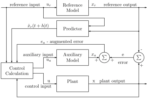
The general adaptive controller structure is depicted in Figure 1. From the figure it is clear that unlike the standard MRAC structure which is widely used in the adaptive control literature for plants without delay, in our feedback path in Figure 1 the augmented error is used instead of the standard errore(t) =x(t)−xr(t). Moreover, in the controller structure the “Adjusted auxiliary model” and “Predictor” blocks are added. The control generator generates the control signalu(t) to the plant and the inputua(t)to the auxiliary model.
V. CONCLUDINGREMARKS
For a class of nonlinear systems with an external dis-turbance and with both input and state delays we utilize the new structure in [16] of adaptive input and state delay compensation based only on lumped delay blocks without so-called distributed-delay (DD) blocks. The design procedure is based on the concept of reference trajectories prediction and the formulation of an augmented error. The model output matching between plant and reference model is accomplished by an adaptive compensator based on the delayed and predicted reference signals and some auxiliary model driven by the signal ua(t) =θω(t)ω(t). Note, that the dynamics of the auxiliary model (14) is exactly the same as the reference model dynamics (2). An appropriate Lyapunov-Krasovskii
P P
-6
-?
-?
6 ?
Reference reference input ur
Model Auxiliary
Plant Control
Calculation
error e
xa
ea- augmented error
+ +
+
-u
ua
xr Model
x
reference output
control input auxiliary input
?
plant output Predictor
ˆ
[image:4.612.317.553.56.216.2]xr(t+h|t)
Fig. 1. The general adaptive controller structure
type functional is introduced for updating the controller parameters and for the stability analysis.
Much more difficult than the problem treated in this paper is the case of nonstable plants. The difficulty is mainly the necessary prediction in the closed loop. One of several possible approaches is to split the overall design in two distinct phases. The first phase addresses the so-called ”robust stabilization problem”, which consists of designing a memoryless state feedback which stabilizes the uncertain system, i.e. the design of a some gainθ#in order to stabilize (1), see e.g. [15]. In the second ”adaptive control design” phase, only the fact that θ# exists is required, see Section 2-4; the exact value ofθ#is not necessary to know.
ACKNOWLEDGEMENTS
This work was supported by the Israel Science Foundation under Grant 588/07.
REFERENCES
[1] H. Wu, “Adaptive robust tracking and model following of uncertain dynamical systems with multiple time delays,”IEEE Transactions on Automatic Control, vol. 49, no. 4, pp. 611–616, 2004.
[2] E. P. Ryan and C. J. Sangwin, “Controlled functional differential equations and adaptive tracking,”Systems & Control Letters, vol. 47, pp. 365–374, 2002.
[3] A. Ilchmann, E. P. Ryan, and S. Trenn, “Tracking control: performance funnels and prescribed transient behaviour,”Systems & Control Let-ters, vol. 54, no. 7, pp. 655–670, 2005.
[4] P. Pepe, “Adaptive output tracking for a class of non-linear time-delay systems,”International journal of adaptive control and signal processing, vol. 18, pp. 489–503, 2004.
[5] S. S. Ge, F. Hong, and T. H. Lee, “Robust adaptive control of nonlinear systems with unknown time delays,”Automatica, vol. 41, pp. 1181– 1190, 2005.
[6] B. M. Mirkin and P. O. Gutman, “Output-feedback model reference adaptive control for continuous state delay systems,” Journal of Dynamic Systems, Measurement, and Control, vol. 125, no. 2, pp. 257–261, 2003, (Special Issue: Time Delayed Systems).
[7] ——, “Output feedback model reference adaptive control for multi-input multi-output plants with state delay,”Systems & Control Letters, vol. 54, no. 10, pp. 961–972, 2005.
[8] P. A. Ioannou and J. Sun,Robust Adaptive Control. New Jersey: Prentice-Hall, 1996.
[10] K. Ichikawa, “Adaptive control of delay system,”International Journal of Control, vol. 41, pp. 1653–1659, 1986.
[11] S. I. Niculescu and A. M. Annaswamy, “An adaptive smith-controller for time-delay systems with relative degree n∗≤2,”System Control Letters, vol. 49, no. 5, pp. 347–358, 2003.
[12] S. Evesque, A. M. Annaswamy, S. Niculescu, and A. P. Dowling, “Adaptive control of a class of time-delay systems,” Journal of Dynamic Systems, Measurement, and Control, vol. 125, no. 2, pp. 186–193, 2003, (Special Issue: Time Delayed Systems).
[13] Y. Jia, H. Kokame, and J. Lunze, “Simultaneous adaptive decoupling and model matching control of a fluidized bed combustor for sewage sludge,” IEEE Transactions on Control Systems Technology, vol. 11, no. 4, pp. 571–577, 2003.
[14] E. L. Mirkin, “Variable structure adaptive system for object with input delay,”Vestnik IA, vol. 5, no. 5, pp. 27–35, 2004, (in Russian). [15] J.-P. Richard, “Time delay systems: an overview of some recent
advances and open problems,”Automatica, vol. 39, no. 10, pp. 1667– 1694, 2003.
[16] B. Mirkin, E. Mirkin and P.-O. Gutman, “ MRAC of linear ststems with input and state delays,”Proc. of the European Control Confer-ence, 2007.
[17] R. Orlov, L. Belkoura, J. Richard, and M. Dambrine, “On identifia-bility of linear time-delay systems,”IEEE Transactions on Automatic Control, no. 8, pp. 1319–1324, 2002.