Algorithmic Exposure and CVA for exotic derivatives

Algorithmic Exposure and CVA for exotic

derivatives

Alexandre Antonov, Serguei Issakov, Serguei Mechkov

Numerix

April 12, 2012

Abstract

We develop the algorithmic approach for Counterparty exposure calculation and automate its application to arbitrary complicated instruments. Assuming that the portfolio is priced by the backward (American) Monte-Carlo method, our approach allows calculating the credit exposure as a pricing by-product, essentially without modifications in the usual pricing procedure. In particu-lar, for the exposure calculation of callable instruments we manage to avoid a cumbersome aggregation of exercise indicators, applying them sequentially in parallel with the main pricing.

We explain how the obtained exposure can be integrated into the Credit Valuation Adjustment (CVA), based on the extension of the pricing model with a Counterparty credit component. The presented approach to the exposure computation is formulated in an arbitrary probability measure. To perform the measure change we use the cross-currency model semantics and calibrate the model to the real-world measure using indexes projections.

1

Introduction

In this paper we propose a unified approach to computing Monte Carlo simu-lated measures for Market Risk and Counterparty Risk. For Market Risk, the corresponding measures are Monte Carlo VaR (Value at Risk) and Expected Shortfall. For Counterparty Risk, we consider two approaches, which are as-sociated with Basel II and Basel III, respectively. The first approach (Basel II) consists of computing what is generally referred to as Counterparty Credit Exposure. Those risk measures include Potential Future Exposures (PFE), Expected Positive Exposures (EPE), and other related risk measures. Coun-terparty Credit Exposure is the maximum amount of money that can be lost

∗_{e-mails: [email protected], [email protected], [email protected]}

if default occurs for Counterparty and/or Self. A more advanced measure of Counterparty Risk, required by Basel III, is Credit Valuation Adjustment (CVA). CVA is an adjustment to the price of any financial instrument due to the possible default of Counterparty and/or Self, which depends on the default probabilities of Counterparty and/or Self.

There are several components of this approach that need to be discussed. In Quantitative Finance, there is consensus about how to compute price. In contrast to that, for Risk computation, there are various approaches used by middle office practitioners, also provided by Risk system vendors, which do not necessarily agree with each other. Some of these approaches do not allow estimating the error they introduce since they are based on non-controllable approximations. There is also the fundamental challenge of growing dimen-sionality when computing advanced Risk measures for non-linear instruments and structured products that require Monte Carlo method for pricing. This is referred to as “Monte Carlo on Monte Carlo” in the Risk industry and “stochas-tic on stochas“stochas-tic” in the Insurance industry.

In this paper we provide a theoretical base that can be used to reconcile various approaches to computing Risk, establishing the Risk computation on the same level of accuracy as the price computation. It provides a common language for the front and middle offices. One of the fundamentals of this approach is the concept of theExposure. Intuitively, exposure is the distribution of prices, rates, or indexes on future dates. We can speak about Exposure-centric analytics, which generalizes the existing Price-centric analytics, as a rigorous framework for computing advanced Market and Counterparty Risk. This also provides a natural way for computing scenarios for Economic Scenario Generators, by adding economic variables to the scenario generation framework. The main subject of the present article is a calculation of exotic portfolio

exposure. One can define it as possible values of the portfolio price at time t

related to different scenarios of the market evolution. There are at least two significantly different approaches to the subject: one is the Scenario approach and the second is the Modeling based one.

A literature on the subject is quite rich. Many authors are contributed here especially during last years. We mention selected books, reviews and ar-ticles, where further references can be found: Canabarro and Duffie (2003), Pykhtin (2005), Cesari et al. (2010), Gregory (2010), Brigo and Capponi (2010), Pykhtin and Rosen (2010), Brigo et al. (2011).

The Scenario based approach can be presented by the following steps. First, we generate a set of markets (scenarios)Mi(t) at timetincluding yield curves,

implied volatilities etc. Then, for each market, we choose a model and calibrate it to the market. Finally we price our portfolio with the calibrated model for each market. If the portfolio contains plain vanilla instruments we do not need to pass by the model and can evaluate the price directly from the generated market. We will concentrate here on exotic deals portfolio which requires model based pricing.

The main drawback of the Scenario based approach is its big computation effort. Indeed, apart from the model construction one needs to price the exotic deals for each scenario. The pricing procedure often involves slow methods

like the Backward Monte Carlo1 _{which is computationally intensive. Another}

difficulty is related to the scenarios generation. There is a large variety of theoretical and phenomenological approaches to the scenario generation which become rather ambiguous for large cross-asset systems. The last shortcoming is that a period from today to the observation time t is out of scope: events like exercises and payments are not taken into account.

The Modeling approach is free of these drawbacks and based on a strict arbitrage-free model properly calibrated to today implied market. We prefer the model generated scenarios due to the following reasons. First, the exotic instrument pricing can be done in a very efficient manner: we need basically only one pricing. Second, the model provides the full time coverage: scenar-ios are available for all the time-steps. Third, the exposure is automatically consistent with the pricing. Finally, the model measure change can deliver the real-world measure taking into account indexes projections.

The key idea of the Modeling approach was developed by Cesari et al (2010). It associates the portfolio exposure with its future price given by an arbitrage-free model. As mentioned above, this approach is very attractive for exotic portfolios while vanilla ones can, in principle, be treated using the Scenarios.

Technically, the Modeling approach reduces to calculation of future portfo-lio prices using Backward Monte Carlo method. This future price is identified with the exposure applying netting conditions. Contrary to the Present Values (PV’s), the exposure distribution depends on the model measure, and practi-tioners often prefer the exposure calculation in a real-world measure. In the article we discuss possibilities of calibration to the real-world measure using a cross-currency model analogy.

For non-callable simple instruments the future price can be calculated an-alytically, or reusing Backward Monte Carlo pricing routines. On the other hand, a callable instrument future price requires a careful calculation of exer-cise conditions and leads to cumbersome modifications of the pricing routines: the Backward pricing calculating exercise condition should be followed by a Forward Monte Carlo aggregating the final result. However, we have managed to include the exposure calculus directly in the Backward pricing routine with-out external changes which leads to a high comfort of the software usage. This is one of our main results in the present article.

The backward pricing procedure including instructions on instruments ex-ecution such as cashflows addition or exercise application is usually written in terms of a pay-off pseudo-code. Our achievement is that the exposure calcula-tion can be done during the backward pricing without changing the pseudo-code structure.

We note here that the Forward Monte-Carlo pricing routine suitable for

pricing of vanillas and semi-exotic instruments is not appropriate for the ex-posure calculation unless analytical methods are available. Indeed, the term exposure refers to a future price, i.e. to conditional expectation of instrument cashflows. Thus an extra mechanism such as analytics or backward Monte Carlo is necessary for the exposure calculation. In the present article we do not

1_{The Backward Monte Carlo method is also referred to in the literature as the Least Squares}

Monte Carlo approach, the Longstaff-Schwartz method [9] or American Monte Carlo one.

consider the forward direction routine but concentrate exclusively on portfolio written and executed in the Backward terms.

A few comments about the concept of a model probability measure. The model calibrated to today market still has an extra degree of freedom – the model stochastic measure. The arbitrage-free theory guarantees that any in-strument present value (PV) does not depend on the measure. However, the

distribution of future prices generated by the model does depend on the mea-sure. Various Risk measures, both for market risk and Counterparty risk (Value at Risk, Potential Future Exposures, etc.) are expressed in terms of these dis-tributions and thus measure dependent. On the other hand, credit valuation adjustment (CVA) is linked with PV’s of default dependent payments and is measure independent. In this work, we assume an arbitrary fixed measure for the model, addressing the real world measure at the end.

The article is organized as follows. Section 2 describes the Modeling ap-proach to the exposure calculation, with several simple illustrations. Section 3

explains our algorithm of the algorithmic exposure calculation for exotic port-folios. Section 4 discusses the CVA computation. Section 5 provides formulas for the risk computation and propose a new method of the real-world mea-sure calibration and usage in the risk estimation. In Section 6 we present the numerical results for simulation in the real world measure.

2

The Modeling approach

Consider a payment of a certain amountAat a dateτ. The present value (PV) of the payment is its discounted expectation

A=E

A

N(τ)

whereN(t) is the model numeraire andE[· · ·] is the pricing expectation in the model measure. We associate the numeraire currency units with domestic ones and require all payments to be expressed in these units.

The paymentseen from some observation datet < τ is a conditional expec-tation

A(t) = E

N(t) A

N(τ)

Ft

Before passing to instrument examples, it is suitable to explain the concept of conditional expectation (CE) E[· · ·| Ft]. Loosely speaking, it is an average

over the stochastic evolution after time t. If we fix the Brownian increments dW(τ) forτ ≤tand average over dW(τ) forτ > t, then our CE is a continuous function of dW(τ) forτ ≤t. On the other hand, for any Markov process, the dependence from the previous Brownian increments is completely absorbed in the Markov state variables. Thus, for any regular path-independent pay-off

P(T) at time T, the discounted CE at time tis a continuous function ofmodel states xi(t)

E

N(t)P(T)

N(T)

Ft

For example, in a hybrid cross-currency setup, the model states can be short rates and FX-rate.

Below we assume the possibility of CE calculation embedded in the Monte Carlo (MC) simulation. A typical numerical method of CE calculation is a

regression to state variables2

E

N(t)P(T)

N(T)

Ft

→X

j

νj βj(x1(t), x2(t),· · ·)

where νj are regression coefficients best fitted in the least-squares sense, and βj(x1(t), x2(t),· · ·) are the basis functions (their choice is the key art of the

method).

2.1

General instrument backward pricing

A general instrument is defined as a payment stream of amountsAj paid at τj

forj = 1,· · ·, M. The amounts are expressed in domestic currency units. They are linked with financial indexes (e.g. Libor, CMS etc.) and, eventually, obey to exercise/barrier conditions.

The instrument today’s price is a PV (discounted expectation) of the pay-ments

V =E 

 M X

j=1

Aj N(τj)





Introduce now the instrumentexposure at certain observation date tobs as

a conditional expectation of future payments w.r.t. the observation date

v=E 

N(t_obs) M X

j=1,τj>tobs

Aj N(τj)

Ftobs



 (1)

Here and below we use the same letter for the price and exposure but capitalize the price notation. Note also absence of time argument in the PV and the exposure notation.

We suppose that the instrument can be calculated using the backward pric-ing procedure also known as pricpric-ing script. The first main object of the back-ward procedure we want to introduce is Continuation Value (CV). It is related with financial products such as legs, options etc. expressed in the domestic cur-rency units. We denote CV’s as Uj(t) with index running over different

prod-ucts. A CV Uj(t) is a certain function of the model state variables at t. Note

also that a unit payment in some currencyXc(t) is itself a CV,UXc(t) =Xc(t). The second main object is a dimensionlessindex which is obtained from the CV’s by two ways

• Ratio (Libor, CMS, FX-rate)

2_{Note that for path-dependent pay-offs the model space is augmented, and the regression}

func-tions should cover the additional dependencies. For example, for asian opfunc-tions where a pay-off depends on a time averagea(t) =Rt

• Indicator (barrier, exercise)

Obviously, an index is a certain function of the model state variables for corre-sponding time.

The backward pricing procedure consist of manipulations with the CV’s on instruments dates (including payment, exercise and trigger dates) and their propagation (a discounted conditional expectation) between the dates. To dis-tinguish these two stages, we use notation Uj(T) for the CV right after the

propagation to the date T and ˜Uj(T) as a result of manipulations of CV’s on

the date T.

All such CV manipulations, or updates, including payments and exercises on an instrument date T can be reduced to the following currency preserving linear combination

˜

Uk(T) = X

m

γm,kUm(T) (2)

whereγm,k are dimensionlessindexes (e.g. numbers, Libors or barrier/exercise

indicators).

The simplest example of such combinations is a swap CV as a difference of fixed and floating legs. Another example is an addition of a payment of index

αn in some currencycn

˜

Un(T) =Un(T) +αnXcn(T)

where Xcn(T) is an exchange rate of the currency cinto domestic currency. Note that a seeming ”non-linearity” may come from the CV dependent indicators. For example, an optimal exercise rule

˜

Uk(T) = max(Um(T), Un(T)) (3)

can be expressed though a linear CV combination with the exercise indicators

˜

Uk(T) =Um(T) 1Um(T)−Un(T)+Un(T) 1Un(T)−Um(T) (4) The discounted conditional expectation between two instrument dates (t < T) reads

Un(t) =E "

N(t) U˜n(T)

N(T)

Ft #

(5)

As mentioned above, the common numerical method to compute the conditional expectation is regression. Note that anupdated CV ˜Un(T) is propagated into a non-updated oneUn(t) on a previous instrument date. One can also interpolate

the CV between the instrument dates t and T: for a date τ, t < τ < T, we simply define the CV as

Un(τ) =E "

N(τ) U˜n(T)

N(T)

Fτ #

Below we consider examples of application of backward pricing procedure to a barrier option, swap, Bermudan option and Autocap. Note that a natural way of pricing of a barrier option and a swap is aForward procedure. However, we cannot use it for the exposure calculation without analytics or other methods giving conditional expectations.

2.2

Instrument examples

2.2.1 Barrier instrument example

Consider a toy barrier instrument paying one unit of currencycat maturityTM

provided that on barrier dates Ti, i= 1,· · ·, M, a rate Li was above a barrier

level B. The rate indexLi is supposed to be a function of model states at Tj.

The payment

Xc(TM) M Y

i=1

1Li>B

at TM gives rise to the PV

V =_E

"

Xc(TM) QM

i=11Li>B

N(TM) #

(6)

In spite of its forward pricing structure, the instrument can be priced backward. Let us denote byV(t) the instrument continuation value (CV) and additionally introduce a CV ˜V(t), an updated version of the CVV(t).

The backward propagation is initialized on the payment date by

V(TM) =Xc(TM)

Then, between two neighboring instrument dates Tj−1, Tj ∈ {T1,· · ·TM} we

repeat the following iterations

• Update CV’s on the barrier datesTj by the indicator3 multiplication

˜

V(Tj) =V(Tj) 1Lj>B (7)

• Calculate discounted conditional expectation atTj−1

V(Tj−1) =E

"

N(Tj−1)

˜

V(Tj) N(Tj)

Ft #

(8)

Note that the update (7) is a special case of the general one (2). The option PV can be obviously obtained asV =V(0).

The instrumentexposure for some observation date tobs < TM is by

defini-tion (1) a discounted conditional expectation

v= E "

N(tobs)

Xc(TM) QM_i=11Li>B

N(TM)

Ftobs

#

(9)

3

Splitting the product into two parts before and after the observation date we obtain

v=

M Y

i=1,Ti≤tobs

1Li>BE

"

N(tobs)

Xc(TM) QMi=1,Ti>tobs1Li>B

N(TM)

Ftobs

#

or

v =V(tobs) M Y

i=1,Ti≤tobs

1Li>B (10)

where

V(t) =E "

N(tobs)

Xc(TM) QM

i=1,Ti>t1Li>B

N(TM)

Ft # (11)

is the instrument CV calculated using the procedure above (7-8). It is easy to see that the instrument exposure is ”path-dependent”.

As mentioned before, the barrier instrument price can be naturally calcu-lated using the Forward Monte Carlo as far as it is presented in terms of a simple average (6). However, its exposure contains conditional averages and cannot be handled using pure Forward Monte Carlo but needs analytics or Backward Monte Carlo.

2.2.2 Swap example

Consider a swap paying a simple non path-dependent index αj in some

cur-rency cj at a date τj for j = 1,· · ·, M. The instrument today’s price is a PV

(discounted expectation) of the payments

S =E 

 M X

j=1

αjXcj(τj)

N(τj) 



Let us refer to a swap CV including the payments after timetasS(t). Introduce also CV ˜S(t), an updated version of the CVS(t) on the payment dates.

Initializing S(TM) = 0 we perform the following backward iterative

proce-dure

• Update swap CV at the payment datesτk adding payment of index4

˜

S(τk) =S(τk) +αkXck(τk)

• Calculate discounted conditional expectation between the payment dates

S(τk−1) =E

"

N(τk−1)

˜

S(τk) N(τk)

Fτk−1 #

4_{As mentioned above the FX-rate is naturally considered a CV expressed in domestic currency}

The swap PV can be obtained asS =S(0). It is easy to see that the swap CV can be expressed via

S(t) =

M X

j=1,τj>t

E

N(t) αjXcj(τj)

N(τj) Ft (12)

The swap exposure sobs for some observation date t is by definition (1) a

conditional expectation

s=E 

N(tobs) M X

j=1, τj>tobs

αjXcj(τj)

N(τj)

Ftobs





which obviously coincides with the swap CV S(t) at timetobs.

2.2.3 Swaption example

Consider a Bermudan swaption giving a right to enter into the swap defined in the previous subsection on exercise dates Ti. The swaption PV is a

dis-counted non-conditional expectation of the payments subjected to theexercise conditions

V =E 

 M X

j=1

I(τj)αjXcj(τj)

N(τj) 



where indicator I(τj) equals to one if we have entered into the swapbefore the

payment dateτj and zero otherwise.

The backward pricing procedure permits calculating the PV and the exercise indicators. Let us denote by V(t) the swaption CV and by ˜V(t) its updated version. Introduce also the instrument days T = {τ1, τ2,· · ·}S{T1, T2,· · ·}, a

union of exercise dates Tj and payment dates τk. The backward pricing is

performed by repeating the steps

• Update CV’s on the instrument dates

˜

V(Tj) = max(V(Tj), S(Tj)) on the exercise dates Tj (13)

˜

S(τk) = S(τk) +αkXck(τk) on the payment dates τk (14)

• Calculate discounted conditional expectation between the neighbor in-strument dates

V(t) =E "

N(t) V˜(T)

N(T)

Ft #

, S(t) =E "

N(t) S˜(T)

N(T)

Ft # (15)

fort, T ∈ T.

We remind that the formulas (15) also define the CV’s for arbitrary times

t falling, for example, between the instrument dates.

The backward pricing procedure (13-15) delivers the swaption today’s price

V(0) along with the exercise indicators. A conditional exercise indicator at time Tj

reflects a trader optimal choice between entering to the swap or continuing with the swaption provided that the swaption was not exercised before. The (unconditional) exercise indicator I(t) can be constructed from the conditional ones

I(t) =Ij for Tj ≤t < Tj+1

where

Ij = 1− j Y

i=1

(1− Ci) (16)

It equals to one if we entered to the swap before or on Tj and zero otherwise.

In other words, a fact that the indicator Ij = 1 means that at least one of

conditional exercise indicators Ci for i= 1,· · ·j was one (obviously, we have a

right to exercise only once).

The swaptionexposure for some observation date tobs is by definition (1) a

discounted conditional expectation

v=E 

N(t_obs) M X

j=1, τj>tobs

I(τj)αjXcj(τj)

N(τj)

Ftobs



 (17)

which can be split in two parts

v=Vco(tobs) (1− I(tobs)) +Vex(tobs)I(tobs)

including continuation partVco(tobs) (the option was not exercised tilltobs) and

exercise part Vex(tobs) (the option was exercised before or on tobs). We can

intuitively identify these parts with the swaption CV and the swap one (12)

v=V(tobs) (1− I(tobs)) +S(tobs)I(tobs) (18)

A formal proof of it is based on the indicators decomposition

Ik= 1− k Y

i=n+1

(1− Ci) !

(1− In) +In for k > n

Indeed, substituting it into the exposure definition (17) fortobs=Tn we obtain

v = E



N(T_n) M X

j=1,τj>Tn

I(Tn, τj)

αjXcj(τj)

N(τj)

FTn



 (1− I_n)

+ E



N(T_n) M X

j=1,τj>Tn

αjXcj(τj)

N(τj)

FTn



 I_n

The first term containing a global exercise indicator conditional to no-exercise beforeTn

I(Tn, τ) = 1− k Y

i=n+1

obviously coincides with the swaption CV V(Tn). Comparing the second term

with the swap CV (12) concludes the proof.

Note that the exposure is a path-dependent product (for callable deals). For example, the continuation partV(tobs) (1−I(tobs)) consists of two contributions.

The first one is the continuation valueV(tobs), i.e. a continuous function of the

model states at the observation date. The second one is the indicator I(tobs)

which is path-dependent, a combination of indicators for exercise dates before the observation.

2.2.4 Autocap example

Autocap is a cap with a limited number of exercises. Namely, we have a right to enterN times into floating-fixed exchanges in domestic currency on a set of dates Ti. Each payment index atTi+1 is defined as

Li−K (19)

where Li is a Libor fixed at time Ti. Thus, the payment as seen at time Ti

equals to

H(Ti) = (Li−K)Pd(Ti, Ti+1) (20)

where Pd(Ti, Ti+1) is a zero bond in domestic currency. For transparency we

limit ourselves to two exercises5 _{N = 2.}

The Autocap pricing is done via a backward induction. Denote two CV’s: the first one corresponds to the product withoneexerciseV(1), while the second oneV(2) _{is a CV of the product withtwoexercises (the instrument to evaluate).}

As usual, we denote the corresponding CV’s with tilde after updates. The backward pricing is performed by repeating the steps

• Update CV’s on the datesTj

˜

V(1)(Tj) = max(V(1)(Tj), H(Tj)) (21)

˜

V(2)(Tj) = max(V(2)(Tj), H(Tj) +V(1)(Tj)) (22)

• Calculate discounted conditional expectation betweenTj−1 and Tj

V(n)(Tj−1) =E

"

N(Tj−1)

˜

V(n)_(T

j) N(Tj)

FTj−1 #

for n= 1,2 (23)

Note that the floating-fixed payment (20) should be treated as a CV: we mul-tiply the CV associated with the zero bond expressed in domestic currency by dimensionless index, Libor minus fixed rate.

The pricing logic is transparent: having two-exercise product we choose to stay with it or exercise into the floating-fixed payment and one-exercise instrument (22). If we have already exercised once, we have V(1) _{and can}

exercise into the floating-fixed payment (21).

5

The iterative procedure which is initialized on TM by V(n)(TM) = 0 for n= 1,2 gives the Autocap PV at origin V =V(2)(0).

Introduce now conditional exercise indicators. The indicatorC_i(2) equals to one if we exercise atTi provided that we have not exercised beforeTi (and zero

otherwise). Analogously, C_i(1) equals to one if we exercise at Ti provided that

we have already exercised once before Ti (and zero otherwise). Obviously, the

indicators can be obtained from the CV’s

C_j(2) = 1_V(2)_(T

j)<H(Tj)+V(1)(Tj) (24)

C_j(1) = 1_V(1)_(Tj)<H(Tj) (25) Using the above indicators, the update rules (21-22) can be rewritten as

˜

V(1)(Tj) = V(1)(Tj) ¯C_j(1)+H(Tj)C(1)_j (26)

˜

V(2)(Tj) = V(2)(Tj) ¯C_j(2)+

H(Tj) +V(1)(Tj)

C_j(2) (27) Before explaining the Autocap exposure we will address unconditional ex-ercise indicators. DenoteI_k(2)an indicator that there was no exercise up to Tk,

inclusively (i.e. it rests two exercises after Tk). Similarly, Ik(1) is indicator of

only one exercise up to Tk, inclusively (i.e. it rests one exercise after Tk). We

call Ek indicator of an exercise atTk (the first or the second).

These global (unconditional) exercise indicators can be obtained using the conditional ones (24-25). Indeed, it is easy to see that no-exercise indicator up to Tk equals to a product of conditional no-exercises

I_k(2) =

k Y

i=1

¯

C_i(2) (28)

where ¯C_i(2)= 1− C(2)_i . The indicator of one exerciseI_k(1) is naturally composed from one conditional exercise C(2) (when we have right for two exercises) and no-exercise after that

I_k(1)=

k X

j=1

j−1

Y

i=1

¯

C_i(2)

!

C_j(2)



 k Y

i=j+1

¯

C_i(1)



 (29)

Finally, the exercise indicator which equals to one if we exercise at Tk is

Ek=C_k(2) k−1

Y

p=1

¯

C_p(2)+

k−1

X

j=1

j−1

Y

i=1

¯

C_i(2)

!

C_j(2)



 k−1

Y

i=j+1

¯

C_i(1)



 C

(1)

k (30)

Its first part corresponds to the first exercise atTkwhile the second one indicates

the second exercise.

Proceed now with the exposure6 _{calculation at observation date t}

obs =Tk.

It is intuitively clear that the exposure is composed of the CV with two exercises

6_{Recall that according to our convention we do not include into the exposure an eventual}

V(2)_(T

k) provided that we have not exercised before (I_k(2) = 1), plus the CV

with one exercise V(1)(Tk) provided that we have exercised once before (I_k(1) =

1), plus the floating-fixed payment at Tk+1 (seen at Tk as H(Tk)) if we have

exercised exactly on Tk, i.e.

v=I_k(2)V(2)(Tk) +I_k(1)V(1)(Tk) +EkH(Tk) (31)

A formal proof of this result is based on a cumbersome but straightforward indi-cators logic, analogous to the Bermudan single-exercise case from the previous section.

3

The exposure calculation

In this section we proceed with exposure calculation for an arbitrary instrument which price can be obtained by the backward induction. As we have seen in the Section2.2.2, an exposure of simple swaps coincides with its continuation value. However, the presence of exercise (callable or barrier instruments) requires more efforts for exposure calculations. Below we will analyze exotic instrument exposure treatment distinguishing two approaches

• Direct

Calculate all components in the backward pricing procedure and assemble them afterwards, by a forward pass

• Algorithmic

Change continuation values operations to obtain the exposure as by-product of the pricing procedure

Note that a good quality conditional expectation (regression) algorithm is essential.

The direct approach algorithm includes the following steps:

• Backward step

Calculate by backward induction and store CV’s (e.g. swap, option etc.) and conditional exercise indicators

• Forward step

Calculate unconditional exercise indicators, for example, using (16) for the bermudan swaption and more complicated logic (28-30) for the Autocap

• Results aggregation

Substitute the obtained components (CV’s and indicators) into final for-mula, for example, (18) for the bermudan swaption and more complicated aggregation (31) for the Autocap

However, the direct exposure calculation approach proposed in Cesari et al. does not treat multi-exercise instruments, for example a call with a barrier trigger or multi-call features. Moreover, it relies on the hierarchical code struc-ture encapsulating before- and after-exercise payment streams, leaving apart stand-alone pricing scripts also presented in financial institutions. For such scripts, the direct exposure calculation approach requires substantial modifi-cations, including both backward and forward steps with a cumbersome logic of exercise indicators calculation and aggregation. It can be very complicated for exotic instruments with different types of exercises like callable instruments with automatic triggers.

Below we propose an alternative, analgorithmic approach to the exposure calculation performed in parallel with the pricing. We suppose that the back-ward pricing procedure includes both essential objects of the ”scripting lan-guage”: continuation values bearing currency units and dimensionless indexes. The idea is to add an extra entity (which we will call Exposure Value) to each Continuation Value. Then, each time we modify the Continuation Value, its Exposure counterpart is also modified according to simple algorithmic rules, giving at origin the product exposure.

Let us describe now the general procedure of the Algorithmic Exposure Cal-culation. We denote by v(t) Exposure Values using small letters to distinguish them from the usual Continuation Values V(t) denoted by capital letters. As usual, we write ˜v(t) for updated Exposure Values.

We assume a complex instrument containing multiple CV’s Um(T) (legs,

swaps, options etc.) and possibly multiple exercise conditions (we have de-scribed various operations with the CV’s in the Sect. 2.1). We recall that the CV’s manipulations are currency unit preserving operations7.

Let us fix an observation datetobs. To calculate exposuresum for all

prod-ucts, we define the corresponding Exposure Values (EV’s) um(T) and their

updated versions after payment, exercise or another combination ˜um(T). The

EV’s calculated at zeroun(0) are closely related with the exposure un. Let us

stress a difference between the product price (being a number) and the exposure (being a stochastic variable).

Along with the CV’s (expressed in domestic currency units and having a continuation sense) the pricing procedure also deals withdimensionless indexes. These objects are obtained as a ratio of two CV’s Un/Um, their comparison

1Un>Um or other dimensionless combinations. In any case the indexes do not have an exposure counterpart.

The EV’s are initialized at the observation date to be equal to the corre-sponding CV’s

um(tobs) =Um(tobs) (32)

The EV’s are kept ”attached” to the CV’s during the further backward propa-gation effectively forming a pair{Um(t), um(t)}fort < tobs.

Now, the unit preserving backward propagation rules (2) and (5) should algorithmicly8 induce the rules for the EV’s fort < tobs

• Linear update rules of the CV’s lead to the same relation with the EV’s

˜

Uk(T) = X

m

γm,kUm(T)

⇓ (33)

˜

uk(T) = X

m

γm,kum(T)

where γm,k are indexes (for example, numbers or barrier exercise

indica-tors)

• No conditional expectation (regression) for the EV’s

Un(t) =E "

N(t) U˜n(T)

N(T)

Ft #

⇓ (34)

un(t) =N(t)

˜

un(T) N(T)

This way, the exposure is finalized once the backward procedure reached the origin

um=um(0)N(tobs)

The algorithmic exposure calculations can be adapted to any backward

pricing script provided that it clearly distinguishes between the dimensionless indexes and the CV’s bearing domestic currency units.

Consider a few practical examples. The first one is related with with optimal exercise update (3) which is equivalent to its ”linearized” version (4). Thus, the maximum update rule of the CV’s induces the following one for the EV’s

˜

Uk(T) = max(Um(T), Un(T))

⇓ (35)

˜

uk(T) =um(T) 1Um(T)>Un(T)+un(T) 1Um(T)≤Un(T)

As another example, consider a payment of an index α in currency c at some date T applied to a legU at timet < tobs

˜

U(t) =U(t) +α Pc(t, T)

where Pc(t, T) is a currency c zero bond converted to domestic currency. A

creation of the zero bond CV Uzb(t) =Pc(t, T) in the r.h.s. will automatically

initialize its EVuzb according to (32)

uzb(t) =

Pc(tobs, T), T > tobs

0, T ≤tobs

The further manipulations with the EV’s in the r.h.s. will lead to

˜

⇓ (36)

˜

u(t) =

u(t) +αPc(tobs, T), T > tobs

u(t), T ≤tobs

As mentioned above, the dimensionless indexes and the CV’s (expressed in domestic currency units) should not be mixed but reflect the nature of the real payments. For illustration set T > tobs. Then, in the purely pricing script we

can formally replace the zero bond Pc(t, T) as the dimensionless index paid

at t in domestic currency. This replace will not change the leg price but will erroneously set the exposure to zero (the payment was formally treated as being done before the observation date).

As the last example, consider the payment date T = t. The general rule (36) gives

˜

U(t) =U(t) +α Xc(t)

⇓ (37)

˜

u(t) =u(t)

where we replace the zero bond in its maturity by the corresponding exchange rate. This means that payments done before the observation do not change the EV and can be ignored.

3.1

Algorithmic exposure calculation: numerical

per-formance

A few words about the method performance in numerical calculations. The computational effort is split between Monte Carlo simulations of model rates and conditional expectation calculation using the Least-Square Monte Carlo. Quite regularly, the latter is much more time consuming than the former. In-deed, it implies intensive calculus with a large number of basis functions, heavy linear algebra and possible nonlinear search procedures. Thus, the main CPU consumption is related with the Least-Square Monte Carlo. The numerical overhead of the algorithmic exposure procedure w.r.t. the pricing is limited to EV’s arithmetic but not with the conditional averages computation which is the most CPU consuming part of the numerics. So we can state that our exposure calculation does not significantly affect the computational effort w.r.t. the usual backward pricing.

3.2

Algorithmic exposure calculation: examples

3.2.1 Barrier instrument example.

Following the general logic we introduce the barrier instrument Exposure Value

In parallel with the main pricing manipulations (7-8) one should execute the following operations with the Exposure Value (EV).

We initialize the EV on the observation date v(tobs) = V(tobs). For dates before the observation datet < tobs the update and roll rules for the EV follow

these of the CV according to the general recipe (33-34) with an indicator as dimensionless index. Putting all together, we have

• The update rules on barrier datesTj Pricing

˜

V(Tj) = V(Tj) 1Lj>B (38)

Exposure

˜

v(Tj) = v(Tj) 1Lj>B (39)

• Roll procedure between the dates

Pricing

V(t) =E "

N(t)V˜(T)

N(T)

Ft #

Exposure

v(t) =N(t)v˜(T)

N(T) (40)

fort, T ∈ {T1,· · ·, TM}. In other words, weskip the conditional

expecta-tion for the exposure calculus.

Finally the exposure equals to

v=v(0)N(tobs) (41)

To see that this expression coincides with the previously obtained one (10) we notice that v(tobs) = V(tobs) on the observation date. Then, combining (39)

with (40) on two barrier neighbor dates we obtain a recursion

v(Tj−1)

N(Tj−1)

= v(Tj)

N(Tj)

1Lj>B (42)

which leads to

v(0)

N(0) =

v(tobs) N(tobs)

M Y

j=1,Tj≤tobs

1Lj>B (43)

3.2.2 Swaption example.

In this section we apply the algorithmic calculation method to the swaption exposure and prove that it coincides with the theoretical result (18).

Introduce EV’s for swaptionv(t) and for swap s(t). We initialize the EV’s on the observation datev(tobs) =V(tobs) ands(tobs) =S(tobs). For datesbefore

the observation datet < tobs the update and roll rules for the EV’s follow these

of the CV’s according to the general recipe (33-34), or, in particular, (35) and (37)

• The update rules on exercise datesTj Pricing

˜

V(Tj) = max(V(Tj), S(Tj))

Exposure

˜

v(Tj) =v(Tj) 1S(Tj)≤V(Tj)+s(Tj) 1S(Tj)>V(Tj) or

˜

v(Tj) = v(Tj) (1− Cj) +s(Tj)Cj (44)

for the exercise indicator Cj = 1S(Tj)>V(Tj).

• Update rules on payment dates τk Pricing

˜

S(τk) =S(τk) +αkXck(τk)

Exposure

˜

s(τk) =s(τk) (45)

• Roll procedure between the dates

Pricing

V(t) = E "

N(t)V˜(T)

N(T)

Ft #

(46)

S(t) = _E

"

N(t)S˜(T)

N(T)

Ft #

(47)

Exposure

v(t) = N(t) ˜v(T)

N(T) (48)

s(t) = N(t) s˜(T)

N(T) (49)

Finally the exposure equals to

v=v(0)N(tobs) (50)

To understand the reason one can compare the option PV

V =E 

 M X

j=1

I(τj)αjXcj(τj)

N(τj) 



with its exposure (1)

v(0) =E 

N(tobs) M X

j=1τj>tobs

I(τj)αjXcj(τj)

N(τj)

Ftobs





Apart from the numeraire the only differences are the conditional expectation of the exposure and absence of the past payments w.r.t. the observation date. That is why we have stopped the regression in the exposure calculation before the observation date along with the payment updates.

Let us prove explicitly that the algorithmic exposure (50) coincides with the previously obtained one (18). Given the swap EV procedures (45) and (49) we have

s(t)

N(t) =

s(tobs) N(tobs)

for t≤tobs

The swaption EV update on the exercise dates (44) combined with its roll rule (48) leads to a recursion

v(Tj−1)

N(Tj−1)

= v(Tj)

N(Tj)

(1− Cj) +

s(tobs) N(tobs)

Cj

for the terminal value v(tobs) = V(tobs). This linear recursion can be easily

solved to obtain the desired expression for the exposure

v=v(0)N(tobs) =V(tobs) (1− I(tobs)) +S(tobs)I(tobs)

Note that a similar recursion logic was applied in Egloff et al (2007) and Andersen-Piterbarg (2010) Sect 18.3.4. in a context of pricing of Callable Libor Exotics. Our contribution is that we explicitly target the exposure and also generalize it for arbitrarily complex instrument.

3.2.3 Autocap example

In this section we apply the algorithmic calculation method to the Autocap exposure and prove that it coincides with the theoretical result (31).

For observation datetobs =Tk introduce EV’s for the underlyings products v(n)_(T

j) and ˜v(n)(Tj) forn= 1,2 and initialize them to the corresponding CV’s v(n)(Tk) =V(n)(Tk) and ˜v(n)(Tk) = ˜V(n)(Tk) (51)

For dates before the observation datet < tobs the update and roll rules for

• Update on the datesTj for j= 1,· · ·, k Pricing

˜

V(1)(Tj) = V(1)(Tj) ¯C_j(1)+H(Tj)C_j(1)

˜

V(2)(Tj) = V(2)(Tj) ¯Cj(2)+

H(Tj) +V(1)(Tj)

C_j(2)

Exposure

˜

v(1)(Tj) = v(1)(Tj) ¯C_j(1)+δjkH(Tk)Cj(1) (52)

˜

v(2)(Tj) = v(2)(Tj) ¯C_j(2)+

δjkH(Tk) +v(1)(Tj)

C_j(2) (53) where the Kronecker delta-symbolδkj = 1k=j in front of the floating-fixed

payment reflects zero EV of the CVH(Tj) forj < k.

• Evolution between the instrument dates

Pricing

V(n)(Tj−1) =E

"

N(Tj−1)

˜

V(n)_(T

j) N(Tj)

FTj−1 #

for n= 1,2

Exposure

v(n)_(T

j−1)

N(Tj−1)

= ˜v

(n)_(T

j) N(Tj)

for n= 1,2 (54)

Finally the Autocap exposure equals to

v=v(2)(0)N(Tk) (55)

Let us prove now that the above algorithmic result coincides with the theory (31). Denoting the discounted values with subscribes,v_j(n) ≡ v(n)(Tj)

N(Tj) and hk =

H(Tk)

N(Tk), and combining (52-53) with (54) we obtain a simple recursion

v_j(1)₋₁ = v_j(1)C¯_j(1)+δjkhkC_k(1) (56) v_j(2)₋₁ = v_j(2)C¯_j(2)+δjkhk+vj(1)

C_j(2) (57)

This system of linear difference equations can be easily solved9 given the terminal valuesv_k(n),n= 1,2. Indeed, substituting the solution of (56)

v_i(1) =v(1)_k k Y

m=i+1

¯

C_m(1)+hkC_k(1) k−1

Y

p=i+1

¯

C_p(1) (58)

into that of (57)

v(2)₀ =v_k(2) k Y

m=1

¯

C_m(2)+

k X

i=1

δikhk+v(1)i

C(2)_i

i−1

Y

p=1

¯

C_p(2) (59)

9_{We used a fact that x}

i = xk Q k

m=i+1 αm+P k

n=i+1 βn Q n₋1

p=i+1αp is the solution of a linear

we obtain

v(2)₀ = v(2)_k k Y

m=1

¯

C_m(2)+v(1)_k k X

i=1

i−1

Y

p=1

¯

C_p(2)C_i(2)

k Y

m=i+1

¯

C(1)_m

+ hk  



C_k(1)

k−1

X

i=1

i−1

Y

p=1

¯

C_p(2)C(2)_i

k−1

Y

p=i+1

¯

C_p(1)+C_k(2)

k−1

Y

p=1

¯

C_p(2)

 



Comparing it with (29-30) we conclude that

v(2)₍₀₎

N(0) =

v(2)_(T

k) N(Tk)

I_k(2)+v

(1)_(T

k) N(Tk)

I_k(1)+H(Tk)

N(Tk)

Ek

which permits to identify the algorithmic Autocap exposure (55) with its ”man-ual” (theoretical) value (31).

4

CVA

Consider now the Credit Valuation Adjustment (CVA) calculation10, see also Cesari et al (2010). We assume the Counterparty credit model be a single-name one with a stochastic intensity. Namely, denote the Counterparty default time by τ. Then the survival process 1t<τ is a Poisson process with some

stochastic intensity (hazard rate) process h(t), see Jeanblanc et al (2009). for more details. The initial pricing model containing arbitrage-free evolution of rates, equities and other market observables is augmented with the hazard rate. The resulting model filtration, i.e. information about the market observables and the hazard rate, is denoted as Ft. Information about the jumps in the

survival process is contained in filtration Dt. Finally, we introduce the whole

filtrationGt=Dt∪Ftassociated with all the information about the market and

the Counterparty survival process. An average over it, E[· · · | Gt], corresponds

to averaging over both jumps and Brownian motions of the rates and the hazard rate.

The main property of the survival process is

E[1T <τ| Gt] = 1t<τE h

e−RtTdu h(u)| F_t

i

(60)

We adopt the ”discount factor” notations for the exponential of the hazard rate integral

H(t) =e−R0tdu h(u) (61) and refer to it as hazard discount factor.

Imagine we receive a payment ofX at timeT, provided that there were no defaults until T. The payment X is assumed to be dependent of the market observable and the hazard rate up to time T, i.e. being measurable w.r.t. the filtration Ft. Then, its PV seen attreads

N(t)E

1T <τ X N(T)| Gt

= 1t<τN(t)E

e−RtTdu h(u) X

N(T)| Ft

. (62)

10

This is the main pricing tool we will use to evaluate default dependent pay-ments.

Proceed now to the CVA calculus. As mentioned before, we should extend our initial pricing model with hazard rate process calibrated to the correspond-ing credit market. Note that the hazard rate evolution can be correlated with the other market observables. After simulation of the extended model we cal-culate the portfolio future values for a fine set of dates Π(t) using the algorithm above. Note that we do not include the credit hazard rates into the regression variables.

Assume also that we have calculated the collateral, C(t), which consists of a certain number Φ(t) of units of some asset A(t) with known (simulated) evolution,

C(t) = Φ(t)A(t).

The Self (”our”) exposure at time tis

O(t) = (Π(t)−C(t))+ leading to the CVA expression

CVA = (1−RRC) Z T

0 E

−d1t<τ

O(t)

N(t)

where RRC is the Counterparty recovery rate which is assumed to be constant.

Indeed, if the Counterparty defaults (d1t<τ =−1) on the interval [t, t+ dt], our

loss will be equal to (Π(t)−C(t))+_{, and this infinitesimal payment, as seen at}

the origin, is equal to the discounted expectation.

Averaging over jumps (independent from the hazard rate)

CVA = (1−RRC) Z T

0 E

−dH(t)O(t)

N(t)

(63)

= (1−RRC) Z T

0

dtE

h(t)H(t) O(t)

N(t)

(64)

reduces to a effective replacement of the survival processes by the hazard ”dis-count factor”

H(t) =e−R0tdu h(u)

Our extended model, containing the market observables and the hazard rate process equipped with the Least Squares MC, is able to compute the above averages. The future portfolio value is calculated as above (the credit hazard rates are not included into the regression variables). The collateral and the hazard discount factor are simulated and the integral element

E

h(t)H(t) O(t)

N(t)

is estimated by averaging.

5

Risk

The risk measure is a general term for statistical characteristics of the instru-ment exposure, i.e. non-discounting (simple) averages

E[f(O(t))]

A simple average is measure-dependent, contrary to the discounted one

E[f(O(t))/N(t)]

which is measure-independent. Here are several examples for the risk-measures

• Potential Future Exposure (PFE) for a confidence level α

qα(t) = inf{x:E[1O(t)<x]≥α}

• Expected Shortfall or Expected Tail Loss

E[O(t)| O(t) > qα(t)]

• Expected Positive Exposure (EPE)

E[O(t)+]

5.1

Right/Wrong way exposure

When the model evolution is highly correlated with the default process the exposure distribution conditional to the default is important, i.e. instead of the CDF of the exposure

CDF(t, x) =E[1O(t)<x]

we need a conditional CDF to default happening at timet

CDFD(t, x) =E[1O(t)<x |τ =t]

where τ is a stochastic default time.

Following our CVA considerations we have

CDFD(t, x) =

E[1O(t)<xd1t<τ] E[d1t<τ]

= E[1O(t)<xh(t)H(t)]

E[h(t)H(t)]

5.2

Real world measure

A model calibrated to today’s market still has an extra degree of freedom – the model probability measure. Usually, we have to fix this measure to be the real-world one for the exposure distribution. The real-world (or physical) probability measure appeared early in Quantitative Finance has not been widely used due to its loose definition, contrary to the risk-neutral measure.

The risk-neutral approach assumes that tradable securities have drift coin-ciding with the short rate r(t). For example, a zero-bond SDE reads

dP(t, T) =P(t, T) (r(t) dt+σ(t) dW(t))

In the ”real world” this drift is supposed to be different but its time-series estimations are vague. We need to link our model to the real-world in a more rigorous way by requiring that some non-discounting (simple) averages hold.

Suppose that we have a set of indices Ij fixed at some times tj and their projections in the futurepj

pj =ERW[Ij]

as expectation in the real-world (RW) measure. Our initial arbitrage-free model in its risk-neutral measure cannot return a priori such averages

pj 6=E[Ij]

Thus we should modify the model measure in order to meet the projections. Note that the model is calibrated to the implied market (initial rates, implied volatilities, etc.) and the only freedom to reproduce the projection is in the measure choice.

To introduce the real-world measure we apply here the cross-currency anal-ogy. Namely, set our initial model as foreign one w.r.t. some FX-rate process and a domestic currency model. Then, our initial model states will get a drift adjustment depending on FX vol and correlations. As a result the initial model in such cross-currency (CC) setup will have a different measure w.r.t. to its risk-neutral one.

To realize the idea we consider a domestic model with a factitious currency ”RW” being a trivial model with zero rates and unit numeraire NRW(t) = 1.

Then we set an FX-rate model between the initial currency and the factitious one to be Black-Scholes (BS) one. Finally a foreign model (initial currency) will coincide with initial model.

The resulting CC model calibration is organized as follows. First, the foreign component (initial model) is calibrated to its implied market. Then, the free parameters, the FX-vol and correlations, are calibrated to meet the indexes projections. This way the calibrated resulting CC model can price the initial instrument (identical to the initial pricing up to numerical errors) and perform the exposure simulation in the real-world measure.

6

Numerical experiments

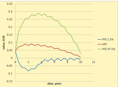
This section is devoted to numerical analysis of the proposed framework. We consider a 10Y cancelable swap: we receive semi-annually a 6M Libor and pay annually a fixed rate (= 2.57%, a swap rate at origin) on 1 EUR notional and we have a right to cancel the swap annually from 4Y. The numerical output is the following.

• 6M Libors expectation in different measures

• distribution (CDF) of 6Y instrument exposure (including the future pay-ments only) in different measures

• exposure profile in the risk-neutral measure

• PFE 97.5% in different measures

The CC Model includes the following components

• Domestic model (RW currency) Trivial model with zero interest rates

• Foreign model (EUR)

Hull-White IR model with 3% rate, 5% mean-reversion and 1.5% volatility

• FX rate (RW currency/EUR)

BS model with correlation with HW Brownian motion ρ=−100% and a set of FX-volatilities: 0%,25%,50%

0 0.02 0.04 0.06 0.08 0.1 0.12

0 2 4 6 8 10 12

Li

b

o

r

a

v

e

ra

g

e

,

%

date,years

fxvol0%

fxvol25%

fxvol50%

0 0.2 0.4 0.6 0.8 1

0.1 0 0.1 0.2 0.3 0.4 0.5

C

D

F

ExposureValue

fx!vol!0%

fx!vol!!25%

fx!vol!50%

0.15 0.1 0.05 0 0.05 0.1 0.15 0.2 0.25 0.3 0.35

0 2 4 6 8 10 12

v

al

u

e

,

E

U

R

date,years

!PFE!2.5%

!EPE

!PFE!97.5%

0 0.05 0.1 0.15 0.2 0.25 0.3 0.35 0.4 0.45

0 2 4 6 8 10 12

v

al

u

e

,

E

U

R

date,years

fxvol0%

fxvol25%

fxvol50%

On the presented graphs we can observe typical shapes of the risk profile. We see that the measure change leads to a positive drift in rates: the bigger FX-vol, the bigger Libor average. We notice significant differences in the exposure distributions in different measures. Thus it is important to use the pricing model in the real-world measure (the factitious CC model should be calibrated to the rates projections) to get the correct exposure distribution.

7

Conclusion

In this article we presented efficient calculations of the portfolio exposure in a self-consistent way using arbitrage-free model calibrated to both implied market and real-world projections. We proposed a new algorithmic method of exposure calculations especially attractive for exotic portfolios avoiding cumbersome ex-ercise aggregation. The new method permits efficient CVA calculation using the simulated information.

In preparing this work, we greatly benefited from the insights of Vladimir Piterbarg. We are grateful to our colleagues at Numerix and especially to Gregory Whitten for providing a stimulating research environment and support.

References

[1] Lief Andersen and Vladimir Piterbarg (2010) ”Interest Rate Modeling”, Atlantic Financial Press

[2] Damiano Brigo and Agostino Capponi, (2010) ”Bilateral counterparty risk with application to CDSs”, Risk Magazine, March 2010

[3] Damiano Brigo, Agostino Capponi, Andrea Pallavicini, and Vasileios Pap-atheodorou (2011), ”Collateral Margining in Arbitrage-Free Counterparty Valuation Adjustment including Re-Hypotecation and Netting”, Available at SSRN

[4] Eduardo Canabarro and Darrell Duffie (2003) ”Measuring and Marking Counterparty Risk”, DefaultRisk

[5] Giovanni Cesari, John Aquilina, Niels Charpillon, Zlatko Filipovic, Gordon Lee, Ion Manda (2010) ”Modelling, Pricing, and Hedging Counterparty Credit Exposure: A Technical Guide”, Springer Finance, Berlin

[6] Daniel Egloff, Michael Kohler, and Nebojsa Todorovic (2007) ”A dynamic look-ahead Monte Carlo algorithm for pricing Bermudan options”, Ann. Appl. Probab. Volume 17, Number 4, 1138-1171

[7] Jon Gregory (2010) ”Counterparty Credit Risk: The new challenge for global financial markets”, Wiley Finance

[8] Monique Jeanblanc, Marc Yor, Marc Chesney (2009) ”Mathematical meth-ods for financial markets”, Springer

[10] Numerix R&D (2010) ”Advanced Risk: Market Risk and Counterparty Credit Risk”, Numerix document

[11] Michael Pykhtin (2005) ”Counterparty Credit Risk Modelling”, Risk books