Quantifying biologically and physically induced flow and tracer dynamics in permeable sediments

under a Creative Commons License.

Quantifying biologically and physically induced flow and tracer

dynamics in permeable sediments

F. J. R. Meysman1, O. S. Galaktionov1, P. L. M. Cook2,*, F. Janssen2, M. Huettel3, and J. J. Middelburg1

1_{Centre for Estuarine and Marine Ecology (CEME), The Netherlands Institute of Ecology (NIOO-KNAW), Korringaweg 7,} 4401 NT Yerseke, The Netherlands

2_{Max Planck Institute for Marine Microbiology, Celsiusstr. 1, Bremen, 28359, Germany} 3_{Department of Oceanography, Florida State University, Tallahassee, FL 32306-4320, USA} *_{now at: CSIRO Land and Water, 120 Meiers Rd Indooroopilly, 4075, Qld, Australia} Received: 20 November 2006 – Published in Biogeosciences Discuss.: 8 December 2006 Revised: 2 August 2007 – Accepted: 8 August 2007 – Published: 9 August 2007

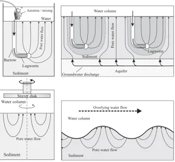
Abstract. Insight in the biogeochemistry and ecology of sandy sediments crucially depends on a quantitative descrip-tion of pore water flow and the associated transport of var-ious solutes and particles. We show that widely differ-ent problems can be modelled by the same flow and tracer equations. The principal difference between model appli-cations concerns the geometry of the sediment-water inter-face and the pressure conditions that are specified along this boundary. We illustrate this commonality with four different case studies. These include biologically and physically in-duced pore water flows, as well as simplified laboratory set-ups versus more complex field-like conditions: [1] lugworm irrigation in laboratory set-up, [2] interaction of bio-irrigation and groundwater seepage on a tidal flat, [3] pore water flow induced by rotational stirring in benthic chambers, and [4] pore water flow induced by unidirectional flow over a ripple sequence. The same two example simulations are performed in all four cases: (a) the time-dependent spread-ing of an inert tracer in the pore water, and (b) the compu-tation of the steady-state distribution of oxygen in the sedi-ment. Overall, our model comparison indicates that model development for sandy sediments is promising, but within an early stage. Clear challenges remain in terms of model de-velopment, model validation, and model implementation.

1 Introduction

Sandy sediments make up a substantial part of coastal and shelf areas worldwide, and consequently, they form an im-portant interface between the aquatic environment and the earth surface (Huettel and Webster, 2001). A prominent characteristic of sandy sediments is their high permeability, which allows pressure gradients to force a flow through the Correspondence to: F. J. R. Meysman

([email protected])

pore spaces. This pore water flow forms an effective trans-port mechanism for various abiotic components, like solutes (Webb and Theodor, 1968) and fine clay particles (Huettel et al., 1996), but also acts as a vector for biological parti-cles, such as bacteria and algae (Rusch and Huettel, 2000). Previous studies have shown that advective transport exerts a major control on sediment biogeochemistry (e.g. Forster et al., 1996; Shum and Sundby, 1996), microbial ecology (e.g. de Beer et al., 2005), and solute exchange across the sediment-water interface (e.g. Huettel et al., 1998). There-fore, our understanding of the biogeochemistry and ecology of sandy sediments crucially depends on a quantitative de-scription of pore water flow and the associated transport of various solutes and particles.

the pore water (Timmermann et al., 2002; Meysman et al., 2006a, b).

In recent years, mathematical modeling has proven a valu-able tool to quantify in-situ flow patterns in sandy sediments and assess their biogeochemical effects (e.g. Rena and Pack-man, 2004; Meysman et al., 2005). Partly, this is because the experimental characterization of solute transport in sandy sediments is challenging for a number of reasons. Firstly, the flow pattern is three-dimensional, while pore pressure and tracer concentrations are typically assessed by point mea-surements. Even with novel tracer imaging techniques, based on arrays of point measurements, it remains very difficult to constrain the flow pattern (Precht and Huettel, 2004; Reimers et al., 2004). A second problem is that tracer measurements cannot be performed without inflicting a significant distur-bance to the sediment. The insertion of electrodes, pla-nar optodes, benthic chambers or other measuring devices into sandy sediment implies that artificial obstacles are intro-duced for the pore water flow and/or that the overlying cur-rents are disturbed. Such a change in boundary conditions might drastically alter the flow pattern within the sediment. Thirdly, the pressure fields that induce pore water flow in sandy sediments are very dynamic by nature. Key physical forcings such as sediment topography, waves and currents can vary dramatically over short time scales (Wheatcroft, 1994; Li and Amos, 1999; Packman and Brooks, 2001). A similar variability also characterizes biologically-induced flow, where bio-irrigating organisms may change their posi-tion and adapt their pumping rate over time scales of minutes to days (Kristensen, 2001). Obtaining representative mea-surements under all likely combinations of these forcings is virtually impossible. Faced with such experimental dif-ficulties, modelling provides a complementary research tool. Models can be used to interpret tracer data obtained from ex-periments, to assess potential distortions introduced by mea-suring devices, or to examine complex field-like conditions that cannot be reproduced in the laboratory.

Nonetheless, models are far from being used as a rou-tine tool in biogeochemical studies of sandy environments, and on the whole, model development is still within an early stage. One aspect that needs attention is the comparison and integration of the existing model approaches for physically and biologically induced solute transport. As noted above, in near-shore sands, both types of processes are important, and may even interact (see below). Typically however, bio-logical and physical aspects have been studied in different re-search communities. Physical mechanisms have attracted the attention of engineers and physicists, focusing on the wave-induced advection below sand ripples (Shum, 1992) and flow over ripples (Savant et al., 1987; Rutherford et al., 1995; El-liott and Brooks, 1997a). As a result of this, a firm mod-elling tradition has been established in the engineering liter-ature (e.g. Rena and Packman, 2004; Cardenas and Wilson, 2006). In contrast, modelling approaches to biologically in-duced flow have only been recently explored, in particular by

marine biogeochemists focusing on the effects of irrigational flows induced by sediment-dwelling organisms (Meile et al., 2003; Meysman et al., 2005, 2006a, b). Overall, these model studies clearly demonstrate the potential of numerical mod-eling to further our understanding of advective transport in sandy sediments. However, model applications differ in the software that is used, the model approximations that are in-corporated, the boundary conditions implemented, and even in the basic model equations (e.g. Darcy versus Brinkman formulation; see discussion below). These differences make cross-system comparisons difficult.

Therefore, it would be valuable to apply a single model approach to different mechanisms of advective flow. Such an integration of physical and biological mechanisms within sandy sediment models was a major focus within two re-cent EU-supported research projects, termed COSA (COastal SAnds as biocatalytic filters; Huettel et al., 2006) and NAME (Nitrate from Aquifers and influences on the carbon cycling in Marine Ecosystems; Postma et al., 2005). For both bio-logically and physically induced pore water flows, the same three-step procedure is adopted, which has emerged over the years as the default strategy to model solute transport in com-plex natural environments (e.g. Elliott and Brooks, 1997a; Rena and Packman, 2004). [a] Process models are devel-oped for a small-scale laboratory benchmark set-up, simulat-ing the pore water flow and the resultsimulat-ing reactive transport. [b] In these simplified set-ups, tracer experiments are carried out under well-controlled conditions, and performance of the process model is validated against these data. [c] When the process model successfully reproduces the benchmark set-up, it can be subsequently extrapolated to simulate flow pat-terns and tracer dynamics in more complex field conditions. For near-shore sandy sediments, the implementation of this (ambitious) scheme is in various stages of progress for the different mechanisms of pore water flow. Here, we report on the current state of model development, validation and appli-cation, reviewing past work as well as providing directions for future research. We show results from four different case studies: [1] lugworm bio-irrigation in laboratory set-up, [2] interaction of bio-irrigation and groundwater seepage on a tidal flat, [3] pore water flows in stirred benthic chambers, and [4] pore water flows induced by unidirectional flow over a sequence of ripples (see overview in Fig. 1). These case studies include both biologically and physically induced pore water flows, as well as simplified laboratory set-ups versus more complex field-like conditions.

2 Model development: pore water flow and reactive transport

ment depth, while the median particle size does not exceed 2 mm (thus excluding gravels). Four different case studies are examined relating to both biologically and physically in-duced flow. In these, we used the same software and we fol-lowed the same procedure to quantify flow patterns and tracer dynamics. This modeling approach consists of two parts. In a first step, the pressure and velocity fields within the pore water are described by a “flow model”. In the development of this “flow model”, the key aspects are the justification of the approximations in the momentum equation, the proper delineation of the model domain, and the selection of the ap-propriate boundary conditions at the boundaries of this model domain. In a second step, the computed velocity field is used as an input for a reactive transport model, which describes the evolution of certain tracer concentrations in the pore water. All model development and simulations are performed using finite element package COMSOL Multiphysics™ 3.2a. The scripts of the various models are freeware, and can be down-loaded from http://www.nioo.knaw.nl/ppages/ogalaktionov/. These model scripts allow the user to adjust model domain geometry, as well as sediment and tracer properties.

2.1 Simplification of the momentum equation

The starting point for model development is the momentum balance for the pore water as derived in multi-phase contin-uum physics (e.g. Bear and Bachmat, 1991). At present, there is some debate on the level of detail that should in-corporated in such a momentum balance, and as a result, existing models differ in their basic flow equation. Khalili et al. (1999) promoted the Darcy-Brinkman-Forchheimer (DBF) equation as a general equation to model pore flow

ρ

₁

φ ∂vd

∂t + 1

φ(vd· ∇)vd

=

−∇p+ρg∇z+ ˜µ∇2vd−

µ kvd−ρ

Cf

√

k

kvdkvd (1)

In this,kdenotes the permeability,µthe dynamic viscosity of the pore water,µ˜ the effective viscosity,ρthe pore water density,Cf a dimensionless drag coefficient,gthe

gravita-tional acceleration, andzthe vertical coordinate. The Darcy velocityvd is related to the actual velocity of pore water as

vd=φv, whereφ is the porosity. In the DBF equation, the

total acceleration (left hand side) balances the forces due to pressure, gravitation, viscous shear stress (Brinkman), linear drag (Darcy), and non-linear drag (Forchheimer). The DBF Eq. (1) has the advantage of generality, but may also engen-der needless complexity. So the question is whether all terms in Eq. (1) are really needed for the applications that are tar-geted. As noted above, we exclusively focus on sands, that is, permeable sediments with a grain diameter less than 2 mm. For sandy sediments, the DBF Eq. (1) can be substantially simplified. Numerical experiments by Khalili et al. (1997)

gibly small in sands. These two terms only become important when pore velocities are really high, like in highly-permeable gravel beds. Accordingly, the momentum balance for sandy sediments readily simplifies to

− ∇p+ρg∇z+ ˜µ∇2vd−

µ

kvd=0 (2)

This so-called Darcy-Brinkman equation forms the basis for the benthic chamber model of Khalili et al. (1997, 1999). However, one issue is whether the Brinkman term is really needed in the momentum equation. Khalili et al. (1999) ar-gued that it should be included to accurately describe advec-tive transport in sands. The Brinkman term is however only important in a transition layer between the overlying water and the sediment, where the velocity profile exhibits strong curvature (∇2vd large). So, the question whether or not to

retain the Brinkman term crucially depends on the thickness δ of this transition layer. Goharzadeh et al. (2005) investi-gatedδ-values for grain sizes from 1 to 7 mm, and found that δroughly equals the grain size diameter. In other words, in sands with a median grain size less than 2 mm, the transition layer is small compared to the scale of the advective flow in-duced by waves, ripples and bio-irrigation, which is on the order of centimeters to decimeters. Accordingly, for practi-cal modeling applications in sandy sediments on the spracti-cale of 10–100 cm depth, the Brinkman and other non-Darcian terms can be justifiably discarded. Note that this cannot be done for applications which specifically target processes within the uppermost surface layer (i.e. the model domain comprises the first few mm of the sediment). An important (and difficult) problem in this respect is the accurate coupling of the flow in the sediment to the free flow over the sediment. As our main focus is the inter-comparison of transport at depth (i.e. well below this surface layer), a detailed discussion of this bound-ary issue is beyond the scope of the present manuscript (see for example the theoretical analysis in Zhou and Mendoza, 1993).

2.2 Flow model

From the viewpoint of the overlying water, the neglect of the small Brinkman transition layer implies that the sediment is regarded as a solid body, and a no-slip boundary condition applies at the sediment-water interface. From the viewpoint of the sediment, it implies that the momentum balance (1) simply reduces to Darcy’s law

vd= −

k

µ(∇p−ρg∇z) (3)

incompressible and that the tracer concentration does not af-fect the densityρ. Then, introducing the effective pressure pe=p−ρgzas the excess pressure over the hydrostatic

pres-sure, one can substitute Darcy’s law (3) into the continuity equation∇ ·vd=0, to finally obtain

∇ ·

−k

η∇pe

=0 (4)

We further assume that the sediment is homogeneous, and so the permeability, porosity, and pore water viscosity remain uniform over the model domain (see Salehin et al., 2004 for a more complex model formulation in heterogeneous sedi-ments). Under the condition of homogeneity, expression (4) reduces to the classical Laplace equation

∇2pe=0 (5)

Appropriate boundary conditions are needed to compute the pressure distribution and the associated pore water velocity field from Eqs. (5) and (3). These boundary conditions differ between individual models and are discussed below. 2.3 Reactive transport model

Once the pore water velocityv is computed, it can be sub-stituted in the mass conservation equation for a solute tracer in the pore water (Bear and Bachmat, 1991; Boudreau, 1997; Meysman et al., 2006)

∂Cs

∂t + ∇ ·(−D· ∇Cs+vCs)−R=0 (6) whereCsdenotes the tracer concentration,Ddenotes the

hy-drodynamic dispersion tensor andR represents the overall production rate due to chemical reactions. Note thatRcan be spatially variable, and that consumption processes are ac-counted for as negative production. The hydrodynamic dis-persion tensor can be decomposed asD=Dmol_+Dmech_, rep-resenting the effects of both molecular diffusion and mechan-ical dispersion (Oelkers, 1996). The part due to molecular diffusion is written as (Meysman et al., 2006)

Dmol=(1−2 lnφ)−1DmolI (7) whereDmol is the molecular diffusion coefficient,I is the unit tensor, and the multiplier(1−2 lnφ)−1forms the cor-rection for tortuosity (Boudreau, 1996). The mechanical dis-persion tensorDmechis given the classical form (Freeze and Cherry, 1979; Lichtner, 1996)

Dmech=DTI+

1

kvk2(DL

−DT)vvT (8)

The quantities DT andDL are the transversal

(perpendic-ular to the flow) and longitudinal (in the direction of the flow) dispersion coefficients, which are expressed as func-tions of grain-scale Peclet numberP e≡dpkvkDmolwhere

dpstands for the median particle size (Oelkers, 1996).

DT =Dmol0.5{P e}1.2 (9)

DL=Dmol0.015{P e}1.1 (10)

The Formulas (9) and (10) are valid for Peclet numbers in the range 1–100, which applies to the models presented here (this was verified a posteriori).

2.4 Implementation and numerical solution

In the simulations presented here, we assume that environ-mental parameters (porosity, permeability, diffusion coeffi-cients) do not vary over the model domain, primarily to fa-cilitate the comparison between models. Spatial heterogene-ity can be important under natural conditions (e.g. the per-meability in a sand ripple can be markedly different from the sediment below), yet its importance for flow patterns and tracer exchange has only been addressed in a few pioneer-ing studies (Salehin et al., 2004), and hence, this is clearly a topic for future research. Furthermore, we assume that changes in the tracer concentration do not significantly influ-ence the pore water properties (density, viscosity). In most cases, this is a realistic assumption that significantly simpli-fies the simulations, as the flow model becomes decoupled from the reactive transport model. Accordingly, the flow model is solved first, and subsequently, the resulting flow field is imported into the reactive transport model. The flow model is implemented using the “Darcy’s Law” mode in the Chemical Engineering Module of COMSOL Multiphysics 3.2a. The reactive transport model is implemented using the “Convection and Diffusion” mode of the same Chemical En-gineering Module. All model parameters can be adjusted in corresponding script files (M-files). These files can be exe-cuted via the MATLAB interface of COMSOL, or they can be run using the newly developed COMSOL Scripts™ pack-age. The usage of scripting allows an easy adjustment of model constants and geometrical parameters.

3 Description of four case studies

Water

Sediment Burrow

Pore water flow

Lugworm

Aeration / mixing Water column

Sediment

Aquifer Groundwater discharge

Pore

water

flow

Lugworm

Water column Stirrer disk

Sediment

Pore water flow

Overlying water flow

Water column

Sediment

Pore water flow

Fig. 1. Schematic representation of the four situations that are modeled: (a) Laboratory incubation set-up commonly used to study lugworm

bio-irrigation; (b) Lugworm bio-irrigation interfering with groundwater seepage on a tidal flat; (c) Pore water flow in stirred incubation chamber; (d) Unidirectional flow over a ripple field inducing pore water flow.

3.1 Bio-irrigation in a laboratory set-up: model [1] Our case study of biological flow focuses on the advec-tive bio-irrigation induced by the lugworm Arenicola ma-rina. Lugworms are abundant in coastal sandy areas world-wide, and are dominant bio-irrigators in these systems (Ri-isg˚ard and Banta, 1998). They inject burrow water at depth, which causes an upward percolation of pore water and seep-age across the sediment-water interface (Timmermann et al., 2002; Meysman et al., 2005). Because of their strong ir-rigational effects, lugworms are frequently used in stud-ies of advective bio-irrigation (Foster-Smith, 1978; Riisg˚ard et al., 1996). Model [1] describes the laboratory incuba-tion set-up (Fig. 1a) that is commonly used to study lug-worm bio-irrigation. Model [1] was proposed in Meysman et al. (2006a) to analyze lugworm incubation experiments with inert tracers. In a follow-up study on model complex-ity, model [1] was compared to a range of simpler and more complex bio-irrigation models (Meysman et al., 2006b).

3.1.1 Problem outline

H

p

H

b

R

b Rc

H

c

Fig. 2. Model [1]: lugworm bio-irrigation in a laboratory core set-up. (a) scheme of the sediment domain geometry and the finite element

mesh; (b) simulated flow line pattern; (c) simulated concentration pattern for the conservative tracer bromide after two hours of flushing;

(d) steady-state concentration pattern of oxygen. Concentrations are expressed relative to the constant concentration in the overlying water

column.

pocket, one can introduce a substantial model simplification (Fig. 2a). Physically, the model domain remains 3-D, but mathematically, it can be described by a radial-symmetric 2-D model that incorporates two variables (the depthzand the distancerfrom the central symmetry axis).

3.1.2 Model domain and boundary conditions

The sediment domain is a cylinder of radiusRs and height

Hs. The injection pocket is represented as a spherical void

of radiusRblocated at the domain’s symmetry axis at depth

Hb. A triangular unstructured mesh was used to discretize

the model domain with a higher resolution near the injection pocket (Fig. 2a). At the lateral sides and the bottom of the incubation core the no-flow condition is adopted. The ac-tual sediment-water interface consists of two parts: the flat sediment surface and the surface of the injection pocket. At the sediment surface, the excess pressure is constant and set to zero, which allows the pore water to leave the sediment domain. Along the surface of the injection pocket the lug-worm’s pumping activity imposes a constant excess pressure pipe . However, no data are available onpeipas this parameter

is difficult to access experimentally. Instead, the lugworm’s pumping rateQis usually reported, which must match the discharge of water across the surface of the injection pocket. When the size of the injection pocket is small compared to both the burrow depthHb and the sediment core radiusRs,

one can directly impose a uniform fluxkvdk =QAipalong

the injection pocket, whereAipis the surface area. When the

injection pocket is small, pressure variations along its surface will be small, and so the flow field that is generated by im-posing a uniform flux will be identical as when imim-posing a constant pressurepipe . When the size of the injection pocket

is relatively large, we implemented a two-step procedure to derive the requiredpefpvalue from the known pumping rate

Q. First, the flow field is calculated for some trial valuep_etest and the associated dischargeQtestis evaluated. Then due to the linearity of Darcy’s law, the pressurepipe corresponding

to the actual fluxQis simply calculated as

peip=pteste

Q

Qtest (11)

Both types of boundary conditions options (small and large injection pockets) are implemented as alternative options in the M-file, which contains the model script.

Fig. 3. Model [2]: interaction between lugworm bio-irrigation and upwelling groundwater on a tidal flat. (a) Sediment domain geometry and

flow line pattern. The bold dashed line separates marine conditions (injection of overlying sea water by the lugworm) and fresh conditions (ground water upwelling from below); (b) simulated concentration pattern for the conservative tracer bromide at steady state; (c) steady-state concentration pattern of oxygen. Concentrations are expressed relative to the constant concentration in the overlying water column.

3.2.1 Problem outline

In recent decades, there is an increased transfer of nitrate from terrestrial areas with intense agriculture to the coastal zone. This results in the eutrophication of coastal waters, causing algal blooms and deterioration of water quality, with significant effects on biodiversity and ecosystem functioning. The default assumption is that most nitrate reaches the sea via riverine input, yet an unknown quantity percolates through the seabed as nitrate-rich groundwater. To this end, the dis-charge of nitrate-bearing groundwater into Ho Bay (Wadden Sea, Denmark) was investigated within the multi-disciplinary EU-project NAME (Postma, 2005). The tidal fluctuation in Ho Bay is about 1.5 m, and ground water (nitrate∼0.6 mM, no sulfate) percolates up through the sandy beach at local-ized sites within the intertidal area (nitrate∼0.03 mM, sul-fate 20 mM).

Within the upper centimeters of the sediment, the groundwater-derived nitrate comes into contact with fresh or-ganic matter, originating from primary production within the bay. Because of the high nitrate concentrations, one would expect that denitrification would be the dominant pathway of organic matter mineralization within the surface sediment. Although high denitrification rates were measured, an in-triguing observation was that the sediment also contained high pyrite concentration, thus indicating sulfate reduction (G. Lavik, personal communication). This would imply that two parallel pathways of organic matter processing are ac-tive: a terrestrial (using nitrate from ground water) along a marine (using sulfate from the overlying seawater). Based on

thermodynamic free-energy constraints and bacterial physi-ology, denitrification and sulfate reduction are mutually ex-clusive, and therefore, a proper explanation was needed to reconcile the occurrence of these two parallel pathways.

One hypothesis that was forwarded as a possible expla-nation focused on the interaction between lugworm bio-irrigation and the upwelling of groundwater. Lugworms are the dominant macrofauna species in the Ho Bay intertidal area where groundwater seepage occurred, with densities up to 25 ind. m−2. The injection of overlying seawater by these lugworms could create marine micro-zones within an other-wise freshwater dominated sediment (Fig. 1b). To investi-gate this effect, model [2] was newly developed (in contrast to model [1], model [2] has not been previously reported in literature).

3.2.2 Model domain and boundary conditions

Similar to model [1] we consider a cylindrical sediment do-main (Fig. 3a). Rather than a laboratory core, this model domain now represents the territory of a single lugworm on the Ho Bay field site. The domain radius can be cal-culated as Rs=(N π )−

1

boundary of the model domain (depth 50 cm). The interac-tion of this upward flow with the lugworm’s irrigainterac-tion leads to a different flow pattern. An upward velocity of 0.3 cm h−1was specified at the lower boundary, based on field ob-servations. As a result, the groundwater flow from below (120 cm3h−1)is two times larger than the lugworm’s pump-ing rate (60 cm3h−1).

3.3 Pore water flow in a benthic chamber: model [3] In our case study of physically induced flow, we focus on the consequences of unidirectional currents over ripple fields. To get a better control on experimental conditions, Huettel and Gust (1992a) proposed a benthic chamber set-up that mimics the pressure variations induced by flow over a sand ripple. A rotating disc creates a circular movement in the overly-ing water, and as a result of this rotational flow, radial pres-sure gradients develop that lead to an advective exchange be-tween pore water and overlying water (Fig. 1c). These ben-thic chambers are now frequently used to study the biogeo-chemical effects of sediment-water exchange in sandy sedi-ments (Glud et al., 1996; Janssen et al., 2005b; Billlerbeck et al., 2006). Model [3] describes the pore water flow and tracer dynamics induced within these benthic chambers. It was pro-posed by Cook et al. (2006) to quantify the influence of ad-vection on nitrogen cycling in permeable sediments. Related chamber models were presented in Khalili et al. (1997) and Basu and Khalili (1999), though starting from a more com-plex equation set (see discussion in Sect. 2)

3.3.1 Problem outline

Physically-induced pore water flow originates from pressure gradients at the sediment surface. Accordingly, the critical issue in model development is the representation of the pres-sure distribution at the sediment-water interface. This ap-plies to the benthic chamber system, but also to other types of physically-induced flow (ripples, waves). There are two pos-sible approaches. One approach depends entirely on model-ing: one derives the sought-after pressure distribution from a coupled hydrodynamic model of the water column (e.g. Car-denas and Wilson, 2007). In the benthic chamber, this im-plies that we explicitly model the rotational flow in the over-lying water starting from the basic Navier-Stokes equations of hydrodynamics (Khalili et al., 1997; Basu and Khalili, 1999). The advantage of the modeling approach is that it can always be implemented. An important drawback is that it requires a proper parameterization of a complex flow model in a complex geometry, and when this is not the case, the simulated results may be far from reality. The alternative approach is to rely on experiments and derive an empirical pressure distribution at the sediment surface. In such exper-iments, the sediment surface is replaced by solid wall, and small pressure gauges are inserted (Huettel and Gust, 1992a; Huettel et al., 1996; Janssen et al., 2005a). The resulting

expression for the pressure distribution along the sediment-water interface can be then used as a forcing function for a sediment model. The experimental approach avoids the ap-plication of a complex flow model, but usually such data are simply not available. For the benthic chamber system, the required pressure distributions have been measured (Huettel and Gust, 1992b; Janssen et al., 2005a). Therefore, in model [3], we can follow the experimental approach. In model [4], we will illustrate the modeling approach.

3.3.2 Model domain and boundary conditions

Mimicking the benthic chamber, the model domain consists again of a cylindrical sediment core of radiusRs and height

Hs (Fig. 4a). We assume that the sediment-water interface

is perfectly flat, and that a perfectly radial-symmetric stir-ring pattern establishes in the overlying water. In this sce-nario, the pressure distribution at the sediment surface will be radial-symmetric, and so, the pore water flow and concen-tration patterns within the sediment will show the same sym-metry. Just like in bio-irrigation model [1], the model domain thus receives radial-symmetric 2-D description that incorpo-rates two variables (the depthzand the distancerfrom the central symmetry axis). A triangular unstructured mesh was used to discretize the model domain, with an element size of

∼0.1 mm at the sediment surface, increasing to 2 mm at the lower boundary of the core (Fig. 4a). Along the bottom and the lateral walls, we implemented a no-flux condition. Fol-lowing Cook et al. (2006), we adopted the folFol-lowing pressure relation at the sediment surface

p (r,0)=2p0(ω)

_r

Rs

2

1−1

2

_r

Rs

2!

(12)

wherep0(ω) is the pressure difference between the outer edge and the center of the chamber. The value ofp0(ω) de-pends on the rotation frequencyωof the stirrer disk, and was measured to be 3.5 Pa at 40 rpm and 14.4 at 80 rpm (Biller-beck et al., unpublished results).

3.4 Pore water flow induced in a ripple bed: model [4] Model [3] simulates the benthic chamber, which in itself was introduced as a physical analogue that mimics pore water flow under sand ripples. In contrast, model [4] directly sim-ulates the free flow over the sand ripples that causes pressure variations at the interface with the overlying water, which in turn, induces pore water flow beneath the ripples.

3.4.1 Problem outline

Fig. 4. Model [3]: pore water flow induced in a stirred benthic chamber. (a) geometry of the sediment domain and the finite element

discretization; (b) flow line pattern; (c) bromide concentration pattern after 12 h of incubation with the rotation speed of the stirrer disk set to 40 rpm; (d) steady-state oxygen distribution (at 40 rpm). Concentrations are expressed relative to the constant concentration in the overlying water column.

1997b; Rena and Packman, 2004, 2005). As was discussed for the benthic chamber, the critical component of the model is again the pressure distribution at the ripple surface. As noted earlier, such pressure relations can be obtained from ei-ther modeling or experiments. In model [3], we implemented the latter option, and this is also the approach taken in previ-ous models of ripple-induced flow (Savant et al., 1987; Elliott and Brooks, 1997a; Rena and Packman, 2004, 2005). Here, in model [4], the pressure relation at the ripple surface is ob-tained by modeling the interaction between the overlying wa-ter flow and the ripple using the Navier-Stokes equations of hydrodynamics. A crucial choice in this is whether to rep-resent the flow regime in the overlying water as laminar or turbulent. Until now, studies on advective exchange have ei-ther implicitly or explicitly assumed that the flow regime re-mains laminar (Khalili et al., 1997; Basu and Khalili, 1999; Cardenas and Wilson, 2007). However, when calculating a characteristic Reynolds number under field conditions, using a characteristic range of flow velocities (u=10–100 cm s−1) and ripple heights (Hr=1–10 cm), one finds relatively high

Reynolds numbersRe=(ρuHr)

µin the range from 103to 105. Although the exact transition from laminar to turbu-lent depends on local flow conditions, it usually commences around Reynolds numbers between 5×103and 104. Accord-ingly, under field conditions, a combination of low flow over small ripples may still lead to laminar flow, but high flow velocities over relatively large ripples could definitely gener-ate turbulent conditions. Laminar and turbulent descriptions of the overlying flow differ considerably. Until now, it has not been assessed how the laminar vs. turbulent description of the water column affects the pore water flow and tracer

dynamics in the sediment. To test this, we performed exactly the same simulations with laminar and turbulent models. The laminar flow model is similar to the ripple models of Car-denas and Wilson (2006, 2007), but for some minor details (rounded ripple geometry; implementation of the periodicity of the model domain).

3.4.2 Water column model

The water column has a height Hw=40 cm, and the

direc-tion of the flow is in the direcdirec-tion of the x-axis (from left to right in Figs. 5a and 6a). The upper boundary of the water column is flat (no waves). The lower boundary displays the topography of the sediment-water interface, and consists of a flat bottom section followed by a sequence of identical rip-ples. The flat section is introduced to allow the development of a representative vertical velocity profile, before the flow hits the first ripple. The subsequent ripple sequence is rel-atively long, so that the flow pattern in the overlying water column is well-established and does not change significantly from ripple to ripple. The number of ripples specified by the input parameternr, which in the present examples is set to

10. Each ripple has the shape of an asymmetric triangle with a gentle front slope and steeper back slope. The shape of the ripples is specified by four parameters, which all can be ad-justed. The default values are the following: the ripple length is set toLr=20 cm, the ripple height is set to Hr=2.13 cm,

and the position of the ripple crest is atLmax=15.67 cm. The crests and troughs are rounded: the curvature radius of these rounded corners is set torc=3 cm.

over a relatively small ripple (∼2 cm), resulting in a Reynolds number around 2000. Such a Reynolds number lies in the transition region from laminar to turbulent flow. Under natural conditions, it would most likely lead to turbu-lent flow. The laminar simulation would not apply then, but the results are still useful for comparison purposes. Laminar and turbulent flow regimes are implemented using the “In-compressible Navier-Stokes“ and “k−εTurbulence Model” modules respectively from the Chemical Engineering Mod-ule of Comsol Multiphysics 3.2a. Both models have simi-lar boundary conditions at the upper and right boundary of the model domain. In both laminar and turbulent regimes, the slip/symmetry boundary condition is specified at the up-per boundary (mimicking a free surface). Outflow condi-tions (zero excess pressure) are implemented at the outflow boundary on the right. At the inflow and at the sediment-water interface, different boundary conditions are imple-mented in both laminar and turbulent regimes. In the lam-inar flow model, the power-profileu(y)=umax(y/Hw)0.14is

prescribed at the inflow whereumax=10.3 cm s−1. This pre-scribed profile mimics a fully developed boundary layer, thus reducing transient effects along the ripple sequence. A no-slip boundary condition is prescribed at the sediment – wa-ter inwa-terface. For the turbulent flow regime, a plug velocity profile is specified at the inflow on the left (constant hori-zontal velocityu=umax=10 cm s−1). When the flow is estab-lished after a few ripples, the horizontal velocity at the upper boundary of the water column becomes 10.7 cm s−1. At the sediment-water interface, we implemented the “logarithmic law of the wall” condition available ink−εmodule. 3.4.3 Pore water flow model

The sediment domain is a rectangular two-dimensional “box” of widthLr=20 cm and depthHs=20 cm. It is placed

under a single ripple spanning the distance between two con-secutive ripple troughs. To reduce the (artificial) influence of the outflow section, the sediment “box” is placed under the 7-th ripple (out of 10 ripples in total). The position of the “test” ripple can be adjusted by modifying the appropriate parametermripplein the script. The side and bottom walls of this “sediment box” are set impenetrable to flow.

3.4.4 Numerical issues

The equation system of the k-εturbulence model is strongly non-linear, and its solution consumes far more memory than the laminar flow solution. We encountered problems when solving the k-εturbulence model for a moderate mesh res-olution. The simulation did not lead to convergence with actual parameter values (actual viscosity and density of sea water) and zero-velocity initial conditions. To get around the problem, we used an iterative procedure, where we first artifi-cially increased the dynamic viscosity of the overlying water a 1000-fold. This solution was then used as initial condition

for a simulation with 10 time lower dynamic viscosity. After four iterations, the desired solution was obtained for the true value of the viscosity.

4 Model validation: simulation of inert tracer experi-ments

4.1 Tracer experiments as model validation

In order to arrive at true quantification, the underlying flow and tracer models should be properly validated against exper-imental data. Unfortunately, a fundamental drawback is that it is hard to directly measure the basic hydrodynamic vari-ables that govern the flow pattern (pressure and pore veloc-ity). Although piezoelectric pressure sensors can be placed in the sediment (Massel et al., 2004), these sensors are too large to resolve the cm-scale pressure gradients involved in bio-irrigational or ripple-induced advection. Moreover, such sensors only provide one-dimensional point measurements, while in reality the flow pattern is three-dimensional. To fully capture the geometry of flow pattern, one thus would require a high-resolution array of point measurements at the same resolution as the model. Recently, Cardenas and Wil-son (2007) did just that for laminar flow over ripples. They compared simulations to experimental data for flow, turbu-lence parameters and most importantly, the pressure along the interface of the ripple, which closely fitted the experi-mental data of Elliott and Brooks (1997b).

Lacking direct measurements, researchers have turned to (indirect) tracer methods to visualize the interstitial pore wa-ter flow. Different approaches have been implemented: (1) adding tracer to the overlying water column and examining the tracer distribution in the pore water through sampling ports (e.g. Elliott and Brooks, 1997b), transparant flume walls (e.g. Salehin et al., 2004; Rena and Packman, 2005) or core sectioning (e.g. Rasmussen et al., 1998), (2) saturat-ing the pore water with tracer, and measursaturat-ing the appearance of the tracer in the overlying water (Huettel and Gust, 1992a; Meysman et al., 2006a), (3) adding dyes to localized zones of pore water (spots or layers), and visualizing the migra-tion and dispersion of these dyed patterns (Huettel and Gust, 1992a; Precht and Huettel, 2004; Salehin et al., 2004), and (4) adding tracer to the overlying water, and measuring the decrease of the tracer in the overlying water (e.g. Glud et al., 1996; Salehin et al., 2004).

Fig. 5. Model [4], laminar variant: Unidirectional flow over a ripple field with laminar flow conditions. (a) velocity field in the water

column; (b) flow line pattern and bromide distribution after 12 h; (c) flow line pattern and steady-state oxygen distribution. Concentrations are expressed relative to the constant concentration in the overlying water column.

Fig. 6. Model [4], turbulent variant: Unidirectional flow over a ripple field with turbulent flow conditions. (a) velocity field in the water

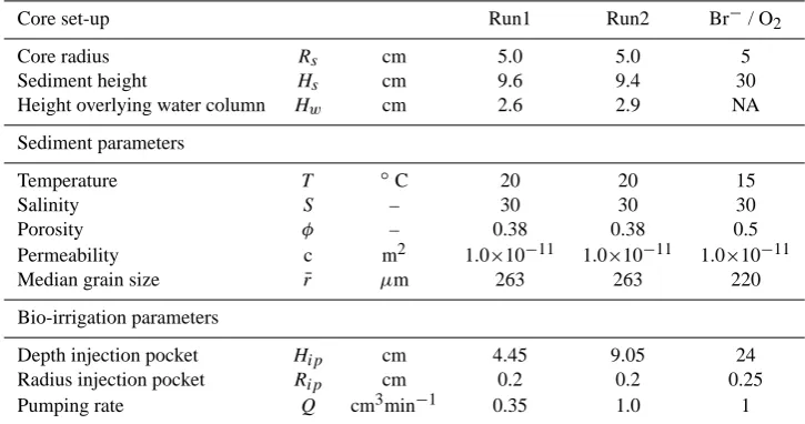
Table 1. Parameter values used in the simulations of lugworm bio-irrigation.

Core set-up Run1 Run2 Br−/ O2

Core radius Rs cm 5.0 5.0 5

Sediment height Hs cm 9.6 9.4 30

Height overlying water column Hw cm 2.6 2.9 NA

Sediment parameters

Temperature T ◦C 20 20 15

Salinity S – 30 30 30

Porosity φ – 0.38 0.38 0.5

Permeability c m2 1.0×10−11 1.0×10−11 1.0×10−11

Median grain size r¯ µm 263 263 220

Bio-irrigation parameters

Depth injection pocket Hip cm 4.45 9.05 24

Radius injection pocket Rip cm 0.2 0.2 0.25

Pumping rate Q cm3min−1 0.35 1.0 1

of flow and tracer models is definitely needed to build up confidence in transport modules of sandy sediment models. When models are able to adequately simulate the advective-dispersive transport of conservative tracers, they can be con-fidently extended to implement more complex biogeochem-istry. Here, we provide an illustration of how this could be achieved for our case studies. Model [1] and [3] describe the flow and tracer dynamics in simplified laboratory set-ups. To test the performance of these models, closed-system incu-bations were conducted with the conservative tracer uranine (Na-fluorescein). A sediment core is incubated with a fixed volume of overlying water, the overlying water is spiked with uranine, and the evolution of the tracer concentration in the overlying water is followed through time. Advective bio-irrigation was examined in cylindrical cores to which a single lugworm was added. Similarly, physically-induced exchange was examined in cylindrical chambers with a recirculating flow imposed in the overlying water. The experimental ap-proach is entirely analogous in the lugworm incubations (re-ferred to as “Exp 1”) and the benthic chamber experiments (referred to as “Exp 2”).

4.2 Model extension: simulation of tracer dynamics in overlying water

Closed-incubation systems have a limited volume of ing water, and hence, the tracer concentration in the overly-ing water will change as a result of the exchange with the pore water. Accordingly, in addition to the pore water flow and reactive transport models for the sediment, one needs a suitable model that describes the temporal evolution of the tracer concentrationCow(t )in the overlying water. For an inert tracer, the total tracer inventory in pore water and over-lying water should remain constant in time

VowCow(t )+ Z

Vs

φCpw(r, z,t ) dVs=

VowC₀ow+ Z

Vs

φC₀pwdVs (13)

whereVs is the volume of the sediment andVow the vol-ume of the overlying water. The initial tracer concentrations in the overlying water and pore water are denotedC₀ow and C₀pwrespectively. The mass balance [13] can be re-arranged into an explicit expression for the tracer concentration in the overlying water column:

Cow(t )=C₀ow+ φ

Vow

Z

Vs

C₀pw−Cpw(r, z,t )dVs (14)

The pore water concentrationCpw(r, z,t )is provided by the reactive transport model. The integral on the right hand side is numerically evaluated by standard integration procedures. Equation (14) then predicts the evolution of the tracer con-centration in the overlying water column. The water column model [14] is coupled to the reactive transport model via the integration coupling variable option in COMSOL Mul-tiphysics 3.2a.

4.3 Experimental methods

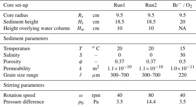
Table 2. Parameter values used in the simulations of the stirred benthic chamber.

Core set-up Run1 Run2 Br−/ O2

Core radius Rs cm 9.5 9.5 9.5

Sediment height Hs cm 18.5 18.5 20

Height overlying water column Hw cm 10 10 NA

Sediment parameters

Temperature T oC 20 20 15

Salinity S – 0 0 30

Porosity φ – 0.37 0.37 0.5

Permeability k m2 1.1×10−10 1.1×10−10 1.0×10−11

Grain size range r¯ µm 300–700 300–700 220

Stirring parameters

Rotation speed ω rpm 40 80 40

Pressure difference p0 Pa 3.5 14.4 3.5

adsorption onto the organic matter coating of sediment parti-cles, clean construction sand was used. Before use, the con-struction sand was washed thoroughly with demineralised water to further remove any remaining organic matter, and thereby reducing background fluorescence as much as pos-sible. Porosity, permeability, solid phase density, and grain size characteristics are presented in Tables 1 and 2.

In the incubations, a core with an inner radiusRswas first

filled with filtered seawater (Exp 1) or tap water (Exp 2). Subsequently, the core was filled to a heightHs by adding

dry sediment. This was done carefully to prevent the trapping of air bubbles within in the sediment. The heightHw of the

overlying water was measured. At the beginning of incuba-tion, the overlying water was spiked with uranine stock solu-tion. Subsequently, the uranine fluorescence in the overlying water was measured continuously with a flow through cell. In Exp 1, uranine was measured at 520 nm using a Turner Quantech Digital Fluorometer (FM 109530-33) with 490 nm as the excitation wavelength. In Exp 2, uranine was deter-mined on a spectrophotometer by measuring absorbance at 490 nm. All experiments were conducted in a darkened room (to prevent degradation of uranine by UV) at a constant tem-perature of 20◦C. Uranine concentrations are expressed rela-tive to the initial concentration immediately after spiking.

In the lugworm incubations (Exp 1), one specimen of Arenicola marina was introduced in the middle of the sed-iment surface of the core and was allowed to burrow. Sub-sequently, the core was left for 48 h in order to allow the lugworm to acclimatize to the new sediment conditions. It was assumed that after this acclimation period, the lugworm had adopted a representative pumping regime. The position of the lugworm in the core was recorded as the burrowing depthHb(measured from the sediment-water interface). The

radius of the injection pocketRbwas estimated after the

ex-periment by sectioning the core after the exex-periment. During

the incubation, the overlying water was aerated and continu-ously kept in motion with a magnetic stirrer.

The set-up of the stirred benthic chambers in Exp 2 is de-scribed by Janssen et al. (2005a) and Cook et al. (2006), ex-cept for the chamber radiusRs, which is 95 mm instead of

100 mm (Table 2). The distance between the lower surface of the stirrer disc and the sediment was 100 mm. Replicate experiments were carried out with stirrer speeds set to 40 and 80 rpm.

4.4 Results: lugworm bio-irrigation

Fig. 7. Validation of the model [1] of the lugworm bio-irrigation.

Comparison of the tracer evolution in the overlying water column with model prediction. The tracer concentration is expressed rela-tive to the initial concentration in the overlying water column.

that is inherent to biological activity. In biogeochemical in-cubations (e.g. oxygen consumption, denitrification), such variability can clearly obstruct the interpretation of measured fluxes and rates. Accordingly, future experimental studies on lugworm bio-irrigation should investigate methods that could reduce temporal variability in lugworm pumping (e.g. fine-tuning the acclimatization period of freshly collected ani-mals, or using mechanical mimics of lugworm pumping in-stead of live organisms)

4.5 Results: benthic chamber exchange

Again two incubation experiments (at 40 and 80 rpm) are shown in Fig. 8, alongside the corresponding model output. Note that the model simulations here contain no adjustable parameters. All parameter values are a priori by measure-ments (Table 2). In both runs, the tracer concentration in the overlying water shows a rapid decrease initially, as tracer rich water is flushed into the sediment and tracer free wa-ter flushed out (Fig. 8). Afwa-ter about 5 h, the rate of tracer dilution decreased significantly reflecting the recirculation

Fig. 8. Validation of the model [3] of the benthic chamber.

Com-parison of the tracer evolution in the overlying water column with model prediction. The tracer concentration is expressed relative to the initial concentration in the overlying water column.

of tracer through the sediment. The modeled concentration changes of tracer generally shows a good agreement to that measured, with the initial slopes of the measured and mod-eled tracer concentrations versus time being indistinguish-able. The greatest deviation between the measured and mod-eled results occurred between 1 and 7 h at the stirring speed of 80 rpm, when the model predicted a greater decrease in the tracer concentration compared to that modeled. This de-viation needs further investigation in future studies. Possible causes for this discrepancy could be (1) the pressure distri-bution at the sediment-water interface and (2) the depth de-pendency of porosity and permeability within the core.

5 Model application: tracer dynamics of Br−and O2

dependent spreading of an inert tracer in the pore water, and (b) the computation of the steady-state distribution of oxygen in the sediment. These benchmark situations are particularly interesting for future work on model validation. The time-dependent spreading of a conservative tracer has been exper-imentally determined in lab studies (e.g. Elliott and Brooks, 1997b) as well as in situ (Precht and Huettel, 2004; Reimers et al., 2004). To date, different inert tracers have been used in studies of advective exchange, such as uranine (Webb and Theodor, 1968; Precht and Huettel, 2004), bromide (Glud et al., 1996), iodide (Reimers et al., 2004) and NaCl (Sale-hin et al., 2004). We implemented the diffusion coefficient for bromide in the example simulations. However, the re-sponse should be representative for any other conservative tracer. Similarly, the influence of advective transport on oxy-gen dynamics is a key research topic in biogeochemical stud-ies of sandy sediments. In recent years, planar optodes have been developed that visualize the two-dimensional O2 distri-bution within sediments. Recently, it has been shown that such optodes have great potential in the study of advective sediments (Precht et al., 2004; Franke et al., 2006). The out-put of the O2 simulation thus enables a direct comparison with such planar optodes images.

Figures 2 to 6 show the output of the benchmark simula-tions for all four models. Each time, the flow line pattern, the output of the transient simulation of Br−, and the steady-state simulation of O2are illustrated. In these simulations, we kept the tracer concentration in the overlying water constant for simplicity. So in contrast to the validation simulations of the previous section, we assume that the water column overly-ing the sediment is well-mixed and sufficiently large not to be affected by the exchange with the sediment. In laboratory incubation experiments of the previous section, this assump-tion was clearly invalid due to the limited volume of overly-ing water. For the inert tracer, the reaction termRvanishes in the reactive transport Eq. (6), and the initial concentration in the pore water is set to zero. In the simulation of oxygen, the consumption rate is modelled by the first-order kinetics

RO₂=−kCO₂ (15)

where the kinetic rate constant is fixed atk=0.26h−1. This implies that O2will be removed from the pore water in ap-proximately 8 h due to aerobic respiration and re-oxidation of reduced compounds formed in anaerobic pathways of or-ganic matter decomposition. Obviously, the kinetic con-stant can be readily adapted, and other expressions for the consumption rate may be easily implemented in the model scripts.

5.1 Lugworm bio-irrigation in a laboratory set-up

Parameter values were taken for a representative lugworm in-cubation experiment (inin-cubation “e” from Rasmussen et al., 1998, which was examined in detail in the modeling papers

parameter values are listed in Table 1). Figure 2b shows the typical shape of the predicted flow line pattern: flow lines first “radiate” from injection pocket in all directions, but then curve upwards. Far above the injection pocket, the flow lines align vertically and eventually they all end at the sediment surface. Figure 2c shows the predicted bromide distribution after two hours of pumping at a constant rate of 1 ml min−1. The injection of tracer at depth creates a subsur-face plume of bromide that expands in time. At time zero, this plume starts as a small sphere around injection pocket, but gradually attains an “egg shape” due to the combination of radial and upward flow. When time progresses, the “egg” becomes more and more elongated in the vertical direction. Note that the bromide concentration changes very sharply at the edge of the plume: inside the concentration is nearly that of the overlying water, while outside, the concentra-tion rapidly decreases to zero. This indicates that advecconcentra-tion clearly dominates dispersion as a transport mode (higher dis-persion would imply a broader fringe). This governance of advection over dispersion in lugworm bio-irrigation was also a central conclusion in the combined experimental-modeling study of Meysman et al. (2006a). After laterally averaging (mimicking the conventional experimental procedure of core sectioning and pore water extraction), the bromide plume will show up as a subsurface maximum in a one-dimensional concentration profile. Such subsurface maxima have been observed in laboratory lugworm incubations (Rasmussen et al., 1998; Timmermann et al., 2002) as well as in field stud-ies of intertidal areas with high lugworm densitstud-ies (Huettel, 1990).

Figure 2d shows the predicted steady-state distribution of oxygen for the same pumping rate. The injection of oxy-genated burrow water into the anoxic sediment creates an oxygenated zone around the injection pocket. The oxy-genated region has again an egg-shape, though the decline of oxygen concentration is far more gradual than in the tran-sient simulation of bromide. The smaller gradient of the O2 concentration is now due to the interplay of reaction and advective transport: traveling along with a confined wa-ter package, the oxygen is gradually consumed within that package. A valid question is how long it takes to establish this steady-state pattern when performing a transient simula-tion. For the imposed decay constantk=0.26h−1, and start-ing with no oxygen in the pore water, the steady-state pattern of Fig. 2d is reached after approximately six hours of steady pumping (this is about the inverse of the decay constant, i.e., 6≈1

0.26).

5.2 Interaction between lugworm bio-irrigation and up-welling groundwater

Javandel and Tsang (1986) provided analytical expressions describing the bell-shaped region of injected water. Our nu-merical flow simulations (Fig. 3a) also predict that the sed-iment domain is effectively separated into two separate re-gions that differ in the origin of their water. Deep layers of sediment are flushed by the upwelling ground water. In the absence of bio-irrigation, this ground water would percolate uniformly towards the sediment-water interface. However, when the lugworm is pumping, it creates a “marine niche” that is filled with overlying sea water (shape of bell-jar turned upside down). The separation between the marine and fresh-water zone is shown in Fig. 3 as the bold dashed line. The marine niche serves as an obstacle to the upward flow of the groundwater. The flow lines of the groundwater are diverted around this obstacle. The resulting compression of the flow lines indicates higher pore water velocities. When compar-ing the flow line pattern in the laboratory core (Fig. 2a) with that in the marine niche (Fig. 3a), one sees that (1) the irriga-tion zone is compressed sideways, and (2) that burrow water penetrates less deep below the injection pocket. These two effects are due to the “collision” of the upwelling groundwa-ter with the marine niche.

The separation of two water types is nicely illustrated in the simulation of the conservative tracer (Fig. 3b). In the simulation, bromide is added to the overlying water, and thus functions as a tracer for marine water. The zone of bromide saturation has also the shape of an inverted bell-jar, and co-incides nicely with the “marine niche” in the flow line pat-tern in Fig. 3a. In the lower part, near the injection pocket, the bromide concentration gradient is very steep. As the in-jected water percolates upwards to the sediment surface, side by side with upwelling ground water, hydromechanical dis-persion increasingly mixes the two water masses, diminish-ing the gradient in the bromide concentration. Thus, along the boundary between the two water masses, some moderate mixing of injected sea water and aquifer water takes place. This smoothening of the concentration gradient visible in Fig. 3c is not a computational artifact due to numerical dis-persion: simulations performed with mesh refinement near the separatrix yield essentially the same pattern. Figure 3c shows the steady-state concentration of oxygen. This pattern is essentially the same as in Fig. 2d (keeping in mind that the sediment domain is deeper and wider in Fig. 3c).

Our model simulations provide a possible explanation for the observed co-occurrence of denitrification and sulfate re-duction within the surface sediment of Ho Bay. The injection of overlying seawater by lugworms creates marine micro-zones within an otherwise freshwater sediment. Within the marine microniche, nitrate concentrations are low and sul-fate concentrations are high, thus enabling sulsul-fate reduction. Outside the microniche, nitrate concentrations are high in the upwelling ground water, thus enabling denitrification upon contact with marine organic matter. When randomly insert-ing a core into the sediment, one may capture both parts of marine and freshwater environments, and hence, one may

ob-serve “apparently” parallel pathways of organic processing, which are in fact spatially separated.

5.3 Tracer dynamics in a benthic chamber

The predicted flow line pattern (Fig. 4b) shows both the mag-nitude (vector arrows) as well as the direction (flow lines) of the pore water flow. Overlying water enters the sediment at the outer part of the core, and in response, pore water is pelled from the central part, in accordance with the dye ex-periments of Huettel and Gust (1992a). The flow lines show that – theoretically – the whole sediment is affected by flow. However, the magnitude of the velocity vectors rapidly de-crease with depth, and so, only the upper 5 cm of the sed-iment are truly affected by advection for a given chamber geometry. The transient simulation of bromide (Fig. 4c) was carried out under similar conditions as in model [1]: constant concentration in the overlying water, initially no bromide in the pore water, stirring frequency 40 rpm, and a simulated time of 12 h. Close to the outer wall of the chamber, the bromide shows the deepest penetration (∼4 cm). The steady-state distribution of oxygen (Fig. 4d) reveals a penetration depth of ∼2 cm near the outer wall (the concentration de-creases to 50% at the depth of 1 cm). This penetration depth matches the range as observed under lab conditions (Huettel and Gust, 1992a), and is much larger than would be expected from diffusive transport alone.

5.4 Tracer dynamics in a ripple bed

through the surface of a single ripple was 3.6 times lower in the laminar case than in the turbulent one.

Figures 5b and 6b show the concentration distribution of passive tracer (Br−)after 12 h of flushing. Deepest penetra-tion of tracer occurs at the inflow zone in the upper part of the front slope, as advection increases the penetration that would normally be seen under diffusive conditions alone. In the outflow zone near the ripple crest, strong advection is act-ing against diffusion, reducact-ing the tracer penetration depth to less than 1 mm. However, this value should be treated with caution, as it is actually an artifact of the fixed concentration condition imposed at the SWI. This creates strong gradients, so that that downward diffusion always will counter upward advection. In reality, the outwelling tracer-free water will di-minish concentrations in the overlying water, and this will prevent any tracer penetration in the outwelling zone. De-spite this, the predicted tracer distribution of bromide shows a good qualitative agreement with tracer patterns observed in flume studies of ripple-induced advection (Huettel et al., 1996; Elliott and Brooks, 1997b).

An important observation is that the tracer penetration depth is markedly different in both regimes (to a depth of 1 cm in the laminar case and to more than 2 cm depth in the turbulent case). The steady-state distribution of the reactive tracer (oxygen) is shown in Figs. 5c and 6c. The O2 pene-tration shows the same trend as for the time-dependent dis-tribution of the conservative tracer. At the upper part of the front slope, the maximum penetration of O2occurs. The oxic sediment layer is on the order of 0.5 cm in the laminar case, and 1 cm in the turbulent case. In the outflow region at the ripple crest, the oxygen penetration depth is reduced, as the water exiting the sediment domain is anoxic. Again, the O2 penetration in the outflow region should not be considered as realistic, because the O2concentration at the SWI is artifi-cially kept constant in the model. To prevent such an artifact, coupled models of tracer transport in both water column and sediment should be explored.

Clearly, the choice between laminar and turbulent flow strongly influences the predicted tracer pattern within the sediment. Pressure gradients at the sediment-water inter-face are higher in the turbulent case, leading to higher pore water flow, a 3.6 times larger exchange with the water col-umn, and more conspicuous tracer distribution (deeper tracer penetration in the inflow zone, and reduced penetration in the outflow zones). Turbulent flow over roughness elements like ripples yields a flow circulation and circulation that pro-duces strong boundary gradients. Therefore, the laminar flow model should be expected to significantly underpredict the flux, as discussed in detail in Elliott and Brooks (1997a, b).

However, a pertinent question is whether the results of the turbulent k-epsilon model are realistic and accurate. We do not compare our solutions with data, and hence the correct-ness of the solutions cannot be ascertained. One indication is the location of the pressure where the main in-flow point

sure maximum, should be located at a distance of four times the bedform height when measured from the ripple crest (En-gel, 1981). Our simulation with the k-epsilon model how-ever shows a much closer position to the crest, indicating that the k-epsilon model does not properly capture the circulation in the lee of the bedform, nor the pressure distribution over the ripple interface. Overall the k-epsilon models seems to poorly perform, and other models such as the k-omega for-mulation (e.g. Yoon and Pattel, 1996) should be explored. Overall, our simulations demonstrate that pore flow within the sediment is very sensitive to the model type chosen for the overlying water, and that close scrutiny of the model out-put is warranted.

6 Conclusion and future prospects

The realisation that advective pore water flow is a signifi-cant process in permeable sediments has greatly complicated our conceptualisation of their biogeochemical functioning. There are numerous possible interactions between biologi-cal and physibiologi-cal forcings, which are virtually impossible to measure in situ and are hard to simulate experimentally. The modeling approach that is proposed here can be used as a useful and complementary tool alongside dedicated measure-ments. Models can provide fundamental insight into perme-able sediment functioning and biophysical forcings, which is key to identifying important variables to measure and assess-ing how experiments, representative for in-situ conditions, should be designed. The model comparison presented here shows that model development is promising, but still within an early stage. Clear challenges remain in model develop-ment, calibration, validation, and implementation.

6.1 Challenges in model development

triangular ripples (Vittal et al., 1977; Shen et al., 1990). Al-ternatively, model predictions of this pressure field have also been obtained for benthic chambers (Khalili et al., 1997) and triangular ripples (Cardenas and Wilson, 2007; this work). Future studies should examine how model predicted pressure fields compare to experimental data (as was done in Carde-nas and Wilson, 2007 for ripples), and address the cause of possible discrepancies. As indicated in Sect. 6.2, a clear is-sue is the choice of a proper model for the free flow above the sediment: laminar versus turbulent, and k-epsilon versus k-omega. Previous model applications have assumed by de-fault that the flow is laminar. Yet, under representative field conditions, the flow may be either in the transition from lam-inar to turbulent, or fully turbulent. Our analysis shows that tracer transport within the pore water is very dependent on the flow regime in the overlying water. Thek−εturbulence model explored here is only a first step to address this is-sue, as we found out that thek−εdoes not behave accurately near the sediment water interface. Accordingly, a true chal-lenge will be to find an adequate turbulent flow model that correctly predicts the pressure distribution at the sediment-water interface of sandy sediments. In this regard, thek−ω first presented by Yoon and Platel (1996) could be promis-ing. Various efforts are ongoing to implement this model into models for unidirectional flow over ripples (A. Packman, M. B. Cardenas, personal communication).

6.2 Challenges in model validation

Model validation is needed to achieve confidence in the be-haviour and predictions of the model. Yet, to date, only a limited number of pioneering studies have carried out an in-depth validation of tracer models in permeable sediments (Salehin et al., 2004; Rena and Packman, 2004; Meysman et al., 2006; Cardenas and Wilson, 2007). Ideally, any given model should be confronted with a suite of dedicated tracer experiments, involving different tracers and various exper-imental conditions. The most simple validation procedure is “water column validation”: it involves the monitoring of the evolution of tracer concentrations in the overlying water. Such a procedure was successfully applied in section 5 for the bio-irrigation set-up and benthic chamber. Although a valuable first test for any model, “water column validation” in itself cannot be considered to a sufficient validation. In a sophisticated parameter sensitivity analysis of sediment in-cubation models, Andersson et al. (2006) recently showed that “water column validation” is a relatively insensitive to most parameters of the sediment model.

Accordingly, methods are needed that allow the measument of the tracer evolution in the pore water. Until re-cently, such methods were merely used to get a qualitative picture of the interstitial flow. For example, in the pioneering study of wave action by Webb and Theodor (1968), fluores-cein was injected into sand ripples, and the rapid reemer-gence of this dye into the overlying water was timed. Yet in

recent years, sophisticated tracer methods have been devel-oped that allow a more quantitative assessment of the pore water flow velocity. Such methods track the evolution of the tracer through the sediment with an array of multiple sen-sors (Precht and Huettel, 2004; Reimers et al., 2004). Until now, an in depth comparison between such tracer data and model predictions has only been carried out in a few pioneer-ing studies (e.g. Salehin et al., 2004), leavpioneer-ing models largely untested and datasets under-explored.

6.3 Challenges in model application

To date, we only know of a few applications in sandy sed-iments where a 2-D or 3-D pore water flow model is cou-pled to a reactive transport model that incorporates complex biogeochemistry, i.e., multiple chemical reactions with non-linear kinetics (Rena and Packman, 2004, 2005; Cook et al., 2006). Clearly, once the transport part of a given model is thoroughly validated, the reactive part model can be ex-tended. Our model [4] explores the interaction between cur-rents and ripple topography, and in future work this can be extended, to investigate how ripple topography affects sedi-ment processes such as denitrification, nitrification and sul-phate reduction. Given that bottom currents and topography change rapidly and frequently, and that they may play an im-portant role in process rates, we suggest that modeling will be vital for the up-scaling of measured local process rates to whole-system budgets in shallow coastal systems.

Acknowledgements. We thank the reviewers M. B. Cardenas and

A. Packman, and the editor T. Battin, for their accurate and con-structive comments, which greatly improved the manuscript. This research was supported by grants from the EU (NAME project, EVK#3-CT-2001-00066; COSA project, EVK#3-CT-2002-00076) and the Netherlands Organization for Scientific Research (NWO PIONIER, 833.02.2002 to J. Middelburg). This is publication 3962 of the Netherlands Institute of Ecology (NIOO-KNAW).

Edited by: T. J. Battin

References

Aller, R. C.: Transport and Reactions in the Bioirrigated Zone, in: The Benthic Boundary Layer, edited by: Boudreau, B. P. and Jor-gensen, B. B., 269–301, Oxford University Press, Oxford, 2001. Andersson, J. H., Middelburg, J. J., and Soetaert, K.: Identifiability and Uncertainty Analysis of Bio-Irrigation Rates, J. Mar. Res., 64, 407–429, 2006.

Basu, A. J. and Khalili, A.: Computation of Flow Through a Fluid-Sediment Interface in a Benthic Chamber, Phys. Fluids, 11, 1395–1405, 1999.