Complex controls on nitrous oxide flux across a large-elevation gradient in the tropical Peruvian Andes

https://doi.org/10.5194/bg-14-5077-2017 © Author(s) 2017. This work is distributed under the Creative Commons Attribution 3.0 License.

Complex controls on nitrous oxide flux across a large-elevation

gradient in the tropical Peruvian Andes

Torsten Diem1,a, Nicholas J. Morley1, Adan Julian Ccahuana Quispe2, Lidia Priscila Huaraca Quispe2, Elizabeth M. Baggs3, Patrick Meir4,5, Mark I. A. Richards1, Pete Smith1, and Yit Arn Teh1,a

1_{School of Biological Sciences, University of Aberdeen, Aberdeen, UK} 2_{Universidad Nacional de San Antonio Abad del Cusco, Cusco, Peru}

3_{The Royal (Dick) School of Veterinary Studies, University of Edinburgh, UK} 4_{School of GeoSciences, University of Edinburgh, Edinburgh, UK}

5_{Research School of Biology, Australian National University, Canberra, Canberra, Australia} a_{formerly at: the School of Geography and Geosciences, University of St Andrews, St Andrews, UK}

Correspondence to:Yit Arn Teh ([email protected])

Received: 23 March 2017 – Discussion started: 30 March 2017

Revised: 19 September 2017 – Accepted: 19 September 2017 – Published: 15 November 2017

Abstract. Current bottom–up process models suggest that montane tropical ecosystems are weak atmospheric sources of N2O, although recent empirical studies from the

south-ern Peruvian Andes have challenged this idea. Here we report N2O flux from combined field and laboratory

ex-periments that investigated the process-based controls on N2O flux from montane ecosystems across a large-elevation

gradient (600–3700 m a.s.l.) in the southern Peruvian An-des. Nitrous oxide flux and environmental variables were quantified in four major habitats (premontane forest, lower montane forest, upper montane forest and montane grass-land) at monthly intervals over a 30-month period from Jan-uary 2011 to June 2013. The role of soil moisture con-tent in regulating N2O flux was investigated through a

manipulative, laboratory-based 15N-tracer experiment. The role of substrate availability (labile organic matter, NO−₃)

in regulating N2O flux was examined through a

field-based litter-fall manipulation experiment and a laboratory-based15N–NO−₃ addition study, respectively. Ecosystems in this region were net atmospheric sources of N2O, with an

unweighted mean flux of 0.27±0.07 mg N–N2O m−2d−1.

Weighted extrapolations, which accounted for differences in land surface area among habitats and variations in flux between seasons, predicted a mean annual flux of 1.27±0.33 kg N2O–N ha−1yr−1. Nitrous oxide flux was

greatest from premontane forest, with an unweighted mean flux of 0.75±0.18 mg N–N2O m−2d−1, translating to a

weighted annual flux of 0.66±0.16 kg N2O–N ha−1yr−1.

In contrast, N2O flux was significantly lower in other

habitats. The unweighted mean fluxes for lower mon-tane forest, monmon-tane grasslands, and upper monmon-tane forest were 0.46±0.24 mg N–N2O m−2d−1, 0.07±0.08 mg N–

N2O m−2d−1, and 0.04±0.07 mg N–N2O m−2d−1,

re-spectively. This corresponds to weighted annual fluxes of 0.52±0.27 kg N2O–N ha−1yr−1, 0.05±0.06 kg N2O–

N ha−1_yr−1_{, and 0.04±0.07 kg N}

2O–N ha−1yr−1,

respec-tively. Nitrous oxide flux showed weak seasonal variation across the region; only lower montane forest showed signif-icantly higher N2O flux during the dry season compared to

wet season. Manipulation of soil moisture content in the lab-oratory indicated that N2O flux was significantly influenced

by changes in water-filled pore space (WFPS). The relation-ship between N2O flux and WFPS was complex and

non-linear, diverging from theoretical predictions of how WFPS relates to N2O flux. Nitrification made a negligible

contri-bution to N2O flux, irrespective of soil moisture content,

in-dicating that nitrate reduction was the dominant source of N2O. Analysis of the pooled data indicated that N2O flux

was greatest at 90 and 50 % WFPS, and lowest at 70 and 30 % WFPS. This trend in N2O flux suggests a complex

Com-prehensive analysis of field and laboratory data demonstrated that variations in NO−₃ availability strongly constrained N2O

flux. Habitat – a proxy for NO−₃ availability under field con-ditions – was the best predictor for N2O flux, with N-rich

habitats (premontane forest, lower montane forest) showing significantly higher N2O flux than N-poor habitats (upper

montane forest, montane grassland). Yet, N2O flux did not

respond to short-term changes in NO−₃ concentration.

1 Introduction

The tropics are the largest source of atmospheric nitrous ox-ide (N2O), accounting for at least half of all global N2O

emissions (Hirsch et al., 2006; Huang et al., 2008; Kort et al., 2011; Nevison et al., 2007; Saikawa et al., 2014). The bulk of tropical N2O emissions come from terrestrial sources, with

the largest emissions arising from agricultural land and un-managed lowland tropical forests (Hirsch et al., 2006; Huang et al., 2008; Kort et al., 2011; Nevison et al., 2007; Saikawa et al., 2014). However, while we have a relatively robust under-standing of the global atmospheric budget as a whole (Hirsch et al., 2006; Huang et al., 2008; Saikawa et al., 2014), our knowledge of regional atmospheric budgets, particularly at the sub-continental scale, is much more limited, due to the constraints imposed by the spatial distribution of existing at-mospheric sampling networks and ground-based, ecosystem-scale sampling efforts (Kort et al., 2011; Nevison et al., 2004, 2007; Saikawa et al., 2014).

In order to predict and model N2O flux at these smaller

(sub-continental) spatial scales, bottom–up emissions inven-tories or process-based models are often used, with emissions estimates constrained by empirical measurements (Werner et al., 2007; Li et al., 2000; Potter et al., 1996; Saikawa et al., 2013). However, these models are only as reliable as the data used to parameterize them; as a consequence, ecosys-tems that are under-represented in the empirical literature or which are poorly understood may be modelled less ac-curately, with knock-on effects for larger-scale emissions es-timates (Saikawa et al., 2013; Teh et al., 2014; Werner et al., 2007). Nitrous oxide dynamics in montane tropical ecosys-tems are particularly poorly understood, because past re-search has concentrated on N2O flux from lowland tierra

firmeforests (Saikawa et al., 2013; Teh et al., 2014; Werner

et al., 2007). Montane ecosystems, however, are important components of many tropical landscapes, and account for a sizeable land area. For example, in continental South Amer-ica, montane ecosystems (>500 m a.s.l.) cover more than 8 % of the land surface (Eva et al., 2004), and play key roles in regional carbon (C), nitrogen (N), and greenhouse gas (GHG) dynamics (Girardin et al., 2010; Moser et al., 2011; Teh et al., 2014; Wolf et al., 2012, 2011). Process-based models predict that N2O fluxes from these montane

en-vironments are lower than those from the lowland tropics (i.e.

<1.0 kg N2O–N ha−1yr−1)(Saikawa et al., 2013; Werner et

al., 2007). However, these models have rarely been tested against empirical data, and several field studies indicate that N2O flux from montane ecosystems can exceed these prior

models’ estimates (Corre et al., 2010; Teh et al., 2014; Veld-kamp et al., 2008). In some instances, N2O flux from

mon-tane ecosystems can in fact approach emissions from lowland forests, begging the question as to whether or not existing models do, in fact, accurately represent flux from these high-elevation ecosystems (Corre et al., 2010; Teh et al., 2014; Veldkamp et al., 2008).

In order to improve our wider understanding of the dynam-ics and biogeochemistry of N2O in montane tropical forests,

we conducted a combined field and laboratory study to inves-tigate the environmental controls on denitrification and N2O

flux across a large-elevation gradient (600–3700 m a.s.l.) in the tropical Peruvian Andes. Prior work from this region in-dicated that montane ecosystems in this area were stronger sources of N2O than predicted by bottom–up process models

(Teh et al., 2014). In particular, lower-elevation premontane and lower montane forests, which account for the majority of the land area in this region (∼54 %), showed emission rates that are on par with lowland tropical forests, suggesting that these ecosystems could be important contributors to re-gional atmospheric budgets (Teh et al., 2014). Nitrous oxide flux appeared to be derived from nitrate reduction (i.e. den-itrification, dissimilatory nitrate reduction to ammonium), and was linked to seasonal variations in climate, with N2O

emissions increasing during the dry season compared to the wet season (Teh et al., 2014). However, contrary to theoret-ical expectations (Davidson, 1991; Firestone and Davidson, 1989; Groffman et al., 2009; Davidson and Verchot, 2000), N2O flux was not directly correlated with soil moisture

con-tent in our field dataset (Teh et al., 2014), raising unresolved questions about the role of seasonal variations in soil mois-ture content in driving N2O flux. We hypothesized that the

weak relationship between N2O flux and soil moisture

con-tent was because soil water-filled pore space (WFPS) – an index of soil moisture and a proxy for soil anaerobiosis – normally fell above the theoretical threshold where N2O flux

was constrained by the availability of anaerobic microsites (i.e. ∼60 % WFPS) in our preliminary dataset (Davidson, 1991; Firestone and Davidson, 1989; Groffman et al., 2009; Davidson and Verchot, 2000; Teh et al., 2014). Even during the dry season, WFPS rarely fell below this threshold value (Teh et al., 2014), allowing other driving variables, such as nitrate (NO−₃), to play a more dominant role in regulating N2O flux (Teh et al., 2014).

In the work presented here, we extended our time series to multi-annual timescales, in order to better understand the role of longer-term climatic variability in modulating N2O flux.

We also conducted a series of manipulative field and lab-oratory experiments to investigate the mechanistic controls on N2O flux in greater detail, and to test hypotheses raised

Furthermore, these manipulative experiments were crucial in helping us interpret our time series of field observations, be-cause prior research indicated that the relationship between individual control variables (e.g. WFPSor NO−₃)and N2O

flux were confounded by the simultaneous action of mul-tiple control variables (Teh et al., 2014). The overarching goals of this research were to investigate how climate and environmental variables regulate N2O flux over multi-annual

timescales; clarify the role of soil moisture as a proximate or distal control on N2O flux; and evaluate the role of key

sub-strates for nitrate reduction (i.e. labile organic matter, NO−₃)

in driving N2O flux. Specifically, we hypothesized the

fol-lowing.

H1 Enhanced N2O flux during the dry season (i.e. during

periods of reduced soil moisture) is due to an increase in N2O flux from nitrification and reduced N2O reduction

during denitrification

H2 N2O flux is poorly correlated with soil water-filled pore

space in situ because soil moisture content does not nor-mally constrain denitrification under field conditions; however, N2O flux is closely correlated with

water-filled pore space when soil moisture content is more limiting for denitrification (i.e.<60 % WFPS)

H3 N2O flux increases proportionately with the availability

of substrates for denitrification (i.e. NO−₃, labile organic matter).

In order to address these three objectives and their atten-dant hypotheses, we quantified N2O flux and

environmen-tal variables from four major habitat types (premontane for-est, lower montane forfor-est, upper montane forest and montane grassland) at monthly intervals over a 30-month period. We also conducted manipulative laboratory experiments that in-vestigated how variations in soil moisture content (WFPS) and NO−₃ availability influenced N2O flux. In addition, we

manipulated labile organic matter availability through a field-based litter-fall manipulation study, recognizing that labile organic matter plays an important role in supplying not only the reducing equivalents for nitrate reduction, but also in-directly providing inorganic N for ammonia oxidation and nitrate reduction via N mineralization (Morley and Baggs, 2010; Blackmer and Bremner, 1978; Davidson, 1991; Fire-stone et al., 1980; Weier et al., 1993).

2 Materials and methods 2.1 Study site

Measurements were conducted on the eastern slope of the Andes in the Kosñipata Valley, Manu National Park, Peru (Fig. 1) (Malhi et al., 2010). This 3.02×106ha (30 200 km2)

region has been the subject of intensive ecological, biogeo-chemical and climatological studies since 2003 by the Andes

Biodiversity and Ecosystem Research Group (or, ABERG; http://www.andesconservation.org), and contains a series of long-term permanent plots across a 200–3700 m above sea level (m a.s.l) elevation gradient that stretches from the west-ern Amazon to the Andes (Malhi et al., 2010). This part of the Andes experiences pronounced seasonality in rainfall but not in air temperature; the dry season extends from May to September and the wet season from October to April (Gi-rardin et al., 2010). Thirteen sampling plots (approximately 20×20 m each) were established at four different habitats across a gradient spanning 600–3700 m a.s.l., including pre-montane forest (600–1200 m a.s.l.;n=3 plots), lower mon-tane forest (1200–2200 m a.s.l.;n=3 plots), upper montane forest (2200–3200 m a.s.l.;n=3 plots), and montane grass-lands (3200–3700 m a.s.l.;n=4 plots; colloquially referred to as “puna”) (Fig. 1). In premontane forest, sampling plots were established in Hacienda Villa Carmen, a 3065 ha bio-logical reserve operated by the Amazon Conservation As-sociation (ACA), containing a mixture of old-growth forest, secondary forest and agricultural plots (Teh et al., 2014). Sampling for soil gas flux was concentrated in the old-growth portions of the reserve. For lower montane and up-per montane forests, sampling plots were established adja-cent to or within existing 1 ha permanent sampling plots es-tablished by ABERG (Teh et al., 2014). Sampling plots were also established in montane grasslands (Teh et al., 2014). To capture a representative range of environmental conditions, mesotope-scale (100 m–1 km scale landforms) topographic features were sampled (Belyea and Baird, 2006). Mesotopic features include ridges, slopes, flats, and a high-elevation basin. The latter two landforms include wet, grassy lawns with no discernible grade, and a peat-filled depression, re-spectively. Summary site descriptions are provided in Ta-ble 1. Data on soil properties were collected as part of this study, while mean annual precipitation is from earlier re-search by ABERG (Girardin et al., 2010).

2.2 Soil–atmosphere exchange

Field sampling was performed over a 30-month period from January 2011 to June 2013 for all habitats except for premon-tane forest. Due to circumstances outside our control, only 24 months of data were collected for premontane forest, with sampling commencing in July 2011. Soil–atmosphere flux was collected monthly, except where flooding or landslides prevented safe access by investigators to the study sites. Gas exchange rates were determined with five replicate gas flux chambers deployed in each of the 13 plots (n=65 flux obser-vations per month). All representative landforms were sam-pled in each habitat (Table 1).

Soil–atmosphere flux of CH4, N2O and CO2 were

deter-mined using a static flux chamber approach (Livingston and Hutchinson, 1995), although only N2O flux is reported here.

Methane and CO2flux are discussed in detail in another

measure-Figure 1.Map of study sites across the Kosñipata Valley, Manu National Park, Peru.

ments were made by enclosing a 0.03 m2 area with cylin-drical, opaque (i.e. dark), two-component (i.e. base and lid) vented chambers with a∼8 L volume. Chamber bases were permanently installed to a depth of approximately 5 cm and inserted>1 month prior to the commencement of sampling, in order to minimize potential artefacts from root mortality following base emplacement (Varner et al., 2003). Cham-ber lids were fitted with small computer case fans to pro-mote even mixing in the chamber headspace (Pumpanen et al., 2004). Headspace samples were collected from each flux chamber over a 30 min enclosure period, with sam-ples collected at four discrete intervals, 7.5 min apart, us-ing a gastight syrus-inge. Gas samples were stored in evacu-ated Exetainers®(Labco Ltd., Lampeter, UK), shipped to the UK by courier, and subsequently analysed for CH4, N2O

and CO2 concentrations with a Thermo TRACE GC

Ul-tra (Thermo Fisher Scientific Inc., Waltham, Massachusetts, USA) at the University of St Andrews. Chromatographic sep-aration was achieved using a Porapak-Q column, and analyte concentrations quantified using a flame ionization detector (FID) for CH4, electron capture detector (ECD) for N2O,

and methanizer-FID for CO2. Instrumental precision was

de-termined by repeated analysis of standards and was better than 5 % for all detectors. Gas flux rates were determined using the R HMR package to plot best-fit lines to the data for headspace concentration against time for individual flux chambers (Pedersen et al., 2010; R Team, 2012). Gas mixing ratios (ppm) were converted to areal flux by using the Ideal Gas Law to solve for the quantity of gas in the headspace

(on a mole or mass basis), normalized by the surface area of each static flux chamber (Livingston and Hutchinson, 1995). Measurements resulting in zero net flux were included in our dataset.

2.3 Environmental variables

To investigate the effects of environmental variables on trace gas dynamics, we determined soil moisture, soil oxygen con-tent in the 0–10 cm depth, soil temperature, and air temper-ature at the time of flux sampling. Volumetric soil mois-ture content was determined using portable soil moismois-ture probes (ML2x ThetaProbe, Delta-T Device Ltd., Cambridge, UK) inserted into the substrate immediately adjacent to each flux chamber (<5 cm from each chamber base; depth of 0– 10 cm). Soil moisture content is reported here as water-filled pore space (WFPS), and is calculated using the measure-ments of volumetric water content and bulk density (Breuer et al., 2000). Soil O2concentration was determined using the

T able 1. Site characteristics. Mean Mean Bulk Soil Ele v ation annual annual density Soil C Mineral soil particle size Flux band temperature precipitation 0–10 cm C :N 0–10 cm 0–10 cm 10–30 cm Plots chambers m a.s.l. Habitat Latitude Longitude ◦C mm g cm − 3 pH 0–10 cm % Clay Silt Sand Clay Silt Sand Landforms n n 600–1200 Premontane forest 12 ◦53 043 00S 71 ◦23 004 00W 20.5 5318 0.38 ± 0.03 ( n = 21) 3.4 ± 0.1 11.3 ± 0.2 7.9 ± 0.5 5.4 ± 0.3 68.8 ± 3.9 25.4 ± 15.9 8.9 ± 1.8 81.0 ± 1.7 10.3 ± 2.5 ridge, slope, flat 3 15 1200–2200 Lo wer montane forest 13 ◦2 056 00S 71 ◦32 013 00W 17.2 2631 0.19 ± 0.03 ( n = 17) 3.4 ± 0.1 14.5 ± 0.2 25.2 ± 1.3 3.6 ± 0.4 67.3 ± 4.2 29.3 ± 4.5 7.2 ± 0.4 83.8 ± 0.8 9.0 ± 0.9 ridge, slope, flat 3 15 2200–3200 Upper montane forest 13 ◦11 024 00S 71 ◦35 013 00W 10.7 1706 0.41 ± 0.02 ( n = 12) 3.9 ± 0.1 16.8 ± 0.4 16.3 ± 1.0 5.1 ± 0.9 57.1 ± 7.9 37.9 ± 8.7 4.4 ± 2.0 46.5 ± 16.2 49.1 ± 18.1 ridge, slope 3 15 3200–3700 Montane grassland 13 ◦07 019 00S 71 ◦36 054 00W 9.3 2200 0.36 ± 0.03 ( n = 27) 4.1 ± 0.1 12.9 ± 0.4 16.0 ± 1.0 2.6 ± 0.2 54.4 ± 3.0 43.0 ± 3.2 n/a n/a n/a ridge, slope, flat, basin 4 20

Resin-extractable inorganic N flux (i.e. ammonium, NH+₄; nitrate, NO−₃)were quantified in all plots using a resin bag approach (Templer et al., 2005; Subler et al., 1995). From August 2011 onwards, ion exchange resin bags (n=15 resin bags per elevation) were deployed in the plant rooting zone (i.e. 0–10 cm depth in premontane forest, lower montane est and montane grasslands; 0–15 cm in upper montane for-est), following established protocols (Templer et al., 2005; Subler et al., 1995). Samples were collected at monthly in-tervals (where possible) for determination of monthly, time-averaged NH+₄ and NO−₃ flux (Subler et al., 1995). For some plots, this sampling frequency was periodically disrupted due to natural hazards (i.e. landslides, river flooding) preventing safe access to the study sites. Resin bags were shipped to the University of Aberdeen after collection from the field, inorganic N was extracted using 2 M KCl and concentra-tions determined colourimetrically using a Burkard SFA2 continuous-flow analyser (Burkard Scientific Ltd., Uxbridge, UK) (Templer et al., 2005; Subler et al., 1995).

2.4 Water-filled pore space manipulation study

We investigated the effects of WFPS on N2O flux derived

from nitrate reduction or nitrification using a15N tracer ex-periment. Soil cores for all habitats were collected from the 0–10 cm depth, and were not fully air-dried nor sieved prior to incubation. Soils were distributed into glass jars and ad-justed to 10 % below the target WFPS values of 30, 50, 70 and 90 %, either by letting the soils partially air-dry or by adding water to them, depending on the WFPS of the soils at the time of collection (n=5 for each15N addition and 3 controls for each WFPS for a total ofn=212; see Table 2). Additional de-ionized water, containing the15N tracers, was subsequently added gravimetrically to raise WFPS to target levels. The exception to this was for the upper montane for-est, where samples were collected from the 0–10 cm depth of the mineral soil, but not from the organic layer. The reason for this is that the mineral soil layer in the upper montane for-est is overlain by a thick organic horizon up to 17 cm deep, consisting of poorly decomposed leaves, roots, and humic materials; very akin to low density peat (Zimmermann et al., 2012, 2009a, b). In contrast, the organic matter in the upper 10 cm soil layer in the other habitats is closely intermixed with the mineral phase, and does not normally constitute a distinct mineral-free horizon. Thus, to sample mineral soil in the upper montane forest, we had to sample beneath this thick organic horizon.

Two different types of15N tracers (30 at. %) were applied to the soils in order to determine the proportion of N2O

de-rived from nitrate reduction and nitrification (Bateman and Baggs, 2005).14N–NH15₄ N–NO3 was used to quantify the

amount of N2O produced by nitrate reduction, while 15N–

NH15₄ N–NO3was used to quantify the amount of N2O

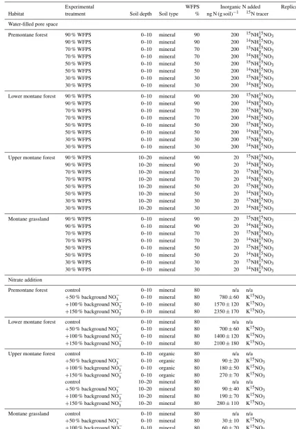
Table 2.Description of the water-filled pore space and NO−₃ addition treatments for the laboratory manipulation experiments.

Experimental WFPS Inorganic N added Replicate

Habitat treatment Soil depth Soil type % ng N (g soil)−1 15N tracer n

Water-filled pore space

Premontane forest 90 % WFPS 0–10 mineral 90 200 15NH15₄NO₃ 5

90 % WFPS 0–10 mineral 90 200 14NH15₄NO₃ 5

70 % WFPS 0–10 mineral 70 200 15NH15₄NO3 5

70 % WFPS 0–10 mineral 70 200 14NH15₄NO3 5

50 % WFPS 0–10 mineral 50 200 15NH15₄NO₃ 5

50 % WFPS 0–10 mineral 50 200 14NH15₄NO3 5

30 % WFPS 0–10 mineral 30 200 15NH15₄NO3 5

30 % WFPS 0–10 mineral 30 200 14NH15₄NO₃ 5

Lower montane forest 90 % WFPS 0–10 mineral 90 200 15NH15₄NO₃ 5

90 % WFPS 0–10 mineral 90 200 14NH15₄NO₃ 5

70 % WFPS 0–10 mineral 70 200 15NH15₄NO3 5

70 % WFPS 0–10 mineral 70 200 14NH15₄NO₃ 5

50 % WFPS 0–10 mineral 50 200 15NH15₄NO₃ 5

50 % WFPS 0–10 mineral 50 200 14NH15₄NO3 5

30 % WFPS 0–10 mineral 30 200 15NH15₄NO3 5

30 % WFPS 0–10 mineral 30 200 14NH15₄NO₃ 5

Upper montane forest 90 % WFPS 10–20 mineral 90 20 15NH15₄NO₃ 5

90 % WFPS 10–20 mineral 90 20 14_NH15

4NO3 5

70 % WFPS 10–20 mineral 70 20 15NH15₄NO3 5

70 % WFPS 10–20 mineral 70 20 14NH15₄NO₃ 5

50 % WFPS 10–20 mineral 50 20 15NH15₄NO₃ 5

50 % WFPS 10–20 mineral 50 20 14NH15₄NO3 5

30 % WFPS 10–20 mineral 30 20 15NH15₄NO3 5

30 % WFPS 10–20 mineral 30 20 14NH15₄NO₃ 5

Montane grassland 90 % WFPS 0–10 mineral 90 20 15NH15₄NO₃ 5

90 % WFPS 0–10 mineral 90 20 14NH15₄NO3 5

70 % WFPS 0–10 mineral 70 20 15NH15₄NO3 5

70 % WFPS 0–10 mineral 70 20 14NH15₄NO₃ 5

50 % WFPS 0–10 mineral 50 20 15NH15₄NO₃ 5

50 % WFPS 0–10 mineral 50 20 14NH15₄NO3 5

30 % WFPS 0–10 mineral 30 20 15NH15₄NO₃ 5

30 % WFPS 0–10 mineral 30 20 14NH15₄NO₃ 5

Nitrate addition

Premontane forest control 0–10 mineral 80 n/a n/a 5

+50 % background NO−₃ 0–10 mineral 80 780±60 K15NO3 5 +100 % background NO−₃ 0–10 mineral 80 1570±120 K15NO₃ 5 +150 % background NO−₃ 0–10 mineral 80 2350±170 K15NO₃ 5

Lower montane forest control 0–10 mineral 80 n/a n/a 5

+50 % background NO−₃ 0–10 mineral 80 700±60 K15NO₃ 5 +100 % background NO−₃ 0–10 mineral 80 1400±120 K15_NO

3 5

+150 % background NO−₃ 0–10 mineral 80 2100±180 K15NO3 5

Upper montane forest control 0–10 organic 80 n/a n/a 5

+50 % background NO−₃ 0–10 organic 80 90±20 K15NO3 5 +100 % background NO−₃ 0–10 organic 80 180±50 K15NO3 5 +150 % background NO−₃ 0–10 organic 80 270±70 K15NO₃ 5

control 10–20 mineral 80 n/a n/a 5

+50 % background NO−₃ 10–20 mineral 80 90±40 K15NO₃ 5 +100 % background NO−₃ 10–20 mineral 80 190±70 K15NO3 5 +150 % background NO−₃ 10–20 mineral 80 280±110 K15NO3 5

Montane grassland control 0–10 mineral 80 n/a n/a 5

of N2O derived from nitrification alone. After application of

the tracers, the jars were sealed and gas samples taken at 0, 6, 12, 24, 36, and 48 h to determine rates of gas flux. Nitrous oxide yield was calculated as the ratio15N–N2O flux :15N–

N2O flux+15N–N2 flux. Soils were sampled at the end of

the experiment for NO−₃ concentration, NH+₄ concentration, and total C and N content.

Soil gas concentrations (N2O, CO2, and CH4)were

mea-sured on a GC as described in Sect. 4.2, while15N–N2and 15_N–N

2O were measured on a SerCon 20 : 20 isotope

ra-tio mass spectrometer equipped with an ANCA TGII pre-concentration module (SerCon Ltd., UK). The coefficient of variation (CV; an index of instrumental precision) for re-peated analysis of gas concentration and isotope standards was <5 %. 15N–N2O and 15N–N2 fluxes were calculated

from the15N atom percent excess of the samples compared to the controls using the HMR package (Pedersen et al., 2010).

2.5 Litter-fall manipulation experiments

We conducted a field-based litter-fall manipulation experi-ment to test for the effects of variations in labile organic mat-ter availability on trace gas flux. This study took place over a 14-month period (April 2012 to June 2013), and consisted of four experimental treatments (control,+50 % litter addition, +100 % litter addition, litter removal) implemented across three habitats (premontane forest, lower montane forest, up-per montane forest), with six replicate plots up-per treatment up-per habitat (each treatment plot was 0.5×0.5 m in size;n=24 observations per habitat; n=72 observations per sampling increment). Leaf litter addition rates for the+50 and+100 % litter addition treatments were determined based on prior re-search from this study site, and fell within the natural range of variability observed across this elevational gradient (Gi-rardin et al., 2010).

Litter-fall for the litter addition treatments was collected monthly in litter baskets (n=3 litter baskets per treatment plot for a total of n = 18 per habitat). These data were also used to determine the background rates of leaf litter-fall among habitats. For the control, litter inputs simply reflected natural background litter-fall rates. For the+50 and+100 % litter addition treatments, background litter inputs were sup-plemented with additional litter taken from the litter baskets. Briefly, wet litter was weighed in the field using a portable scale, gently mixed (homogenized), and then re-distributed to the+50 and+100 % litter addition plots in amounts pro-portional to the average amount of wet litter that fell into the litter baskets over the course of the month. As a consequence, the amount of litter added in the two litter addition treatments was not fixed but varied according to the natural background rate of litter-fall. For the litter removal treatment, leaf litter was removed from the forest floor at the start of the experi-ment, and 3 mm nylon mesh was placed over the surface of the treatment plot to prevent further litter ingress to the soil

surface. Any debris accumulating on the mesh was removed at monthly intervals.

Trace gas flux and environmental variables were deter-mined at seven time points over the course of the 14-month experiment using the methods described in Sect. 4.2. In addi-tion, soil moisture (WFPS from the 0–10 cm depth), soil tem-perature (0–10 cm depth), air temtem-perature, soil gas concen-trations (O2, CH4, N2O, CO2)from the 0–10 and 20–30 cm

depths, litter C, and litter N were determined concomitantly. Litter C and N content was determined on a Carlo-Erba NA 2500 elemental analyser (CE Instruments Ltd, Wigan, UK) at the University of Aberdeen.

2.6 Nitrate addition experiment

To quantify the effect of NO−₃ availability on N2O flux,

we conducted a15N–NO−₃ addition experiment. Background concentrations of NO−₃ were determined prior to the start of the experiment using soil subsamples (n=5 per eleva-tion), after which the soils from each habitat were divided into three treatment groups, and supplemented with surplus NO−₃ which raised these background levels by+50,+100, and+150 % (Table 2). The NO−₃ added to the soil in each of the treatments was enriched with15N in order to trace the conversion of nitrate to gaseous N products (15N–N2O,15N–

N2)(Baggs et al., 2003; Bateman and Baggs, 2005).

Soil cores were sampled from 0–10 cm for each habitat (n=6 soil cores per habitat), with the exception of upper montane forest, where two separate sets of cores were col-lected, one from the organic layer (O horizon;n=6) and the other from the mineral layer (A horizon;n=6). Soil samples were then shipped to the University of Aberdeen and sampled within 1 week of arrival. Transport times from Peru to the UK varied between 1 and 2 weeks. Five of these soil cores, one for each replicate, were split into four equal parts (three treatment samples and one control sample) and distributed into 1 L screw top jars (Kilner, UK). A small soil subsample from each core was used to determine WFPS, background NO−₃ content (extracted in 100 mL 1 M KCl for a 10 g soil sample prior to the start of the experiment), as well as total C and N content. If necessary, the samples were gravimetrically amended with water until the cores reached 80 % WFPS. Soil cores were kept under constant conditions for 3 days before the start of the experiment to minimize the effects of chang-ing water content on soil processes.

At the start of the experiment, dissolved 15N-labelled KNO3 (30 at. %) was added according to the measured

(Table 2). The jars were then sealed with lids fitted with a two-way stopcock to allow for gas sampling. Gas sam-ples were taken with gastight syringes, and stored in pre-evacuated containers for determination of 15N–N2, 15N–

N2O, N2O, CO2, and CH4content. Isotope samples (150 mL)

were stored in 100 mL serum bottles and gas concentration samples (20 mL) were stored in 12 mL Exetainers® (Labco Ltd., Lampeter, UK). After gas sampling, the stopcock was opened to allow the sampled air from the jar to be replaced by lab air, and lab air was sampled to allow for correction of the gas concentrations in the jars due to dilution. Sam-ples were taken at 0, 6, 12, 24, 36, and 48 h, after which the jars were opened and soil was sampled for determination of NO−₃, NH+₄ and total C and N. Gas flux, isotopic and elemen-tal concentrations were determined according to the methods described previously.

2.7 Statistics

Statistical analyses were performed using JMP IN Version 8 (SAS Institute, Inc., Cary, North Carolina, USA) or R (R Team, 2012). Residuals were checked for heteroscedastic-ity and homogeneheteroscedastic-ity of variances. Where necessary, the data were transformed using a Box–Cox procedure to meet the assumptions of analysis of variance. Analysis of variance (ANOVA) or generalized linear models were used to evaluate the effect of categorical variables (i.e. site, season, topogra-phy) on trace gas flux and environmental variables. Analy-sis of covariance (ANCOVA) was performed on Box–Cox transformed data to investigate the combined effects of cate-gorical variables and environmental factors (e.g. water-filled pore space, soil oxygen content, air temperature, soil temper-ature) on trace gas flux. Non-parametric tests were employed where Box–Cox transformation was unable to normalize the data or homogenize the variances, or where the residuals still showed strong trends even after Box–Cox transforma-tion. Means comparisons were performed using Fisher’s least significant difference test (Fisher’s LSD). Statistical signif-icance was determined at the P <0.05 level unless othwise noted. Values are reported as means and standard er-rors (±1 SE). Statistical analyses for the field data were con-ducted on plot-averaged data to avoid pseudo-replication.

3 Results

3.1 Variations in N2O flux among habitats and between seasons

The overall mean N2O flux for the entire dataset was

0.27±0.07 mg N–N2O m−2d−1, with a range from −8.40

to 75.0 mg N–N2O m−2d−1. We investigated the effect of

habitat, season, topography, and the interaction of habitat by season on N2O flux by using a three-way ANOVA on

plot-averaged data (F10,307=3.28,P <0.0005; Supplement

Ta-ble S1a). We found that there was a significant effect of

habi-tat (P <0.003) and an effect of season at the borderline of statistical significance (P <0.07). However, we found no ef-fect of topography and no habitat by season interaction efef-fect on N2O flux. Habitat accounted for the largest proportion of

variance in the dataset (4.3 %), while season accounted for only 1.0 % of the variance (Supplement Table S1a).

Among habitats, the overall trend was towards the highest flux from premontane forest (0.75±0.18 mg N– N2O m−2d−1), followed by lower montane forest

(0.46±0.24 mg N–N2O m−2d−1), montane grasslands

(0.07±0.08 mg N–N2O m−2d−1), and upper montane

forest (0.04±0.07 mg N–N2O m−2d−1)(Fig. 2a). Multiple

comparisons tests indicated that only premontane forests showed statistically higher flux than the others (Fisher’s

LSD,P <0.05); while there were numerical differences in

mean flux among the other habitats, large variances meant that they had overlapping ranges of flux (Fig. 2a).

The borderline significant effect of season (P <0.07) reflected an overall trend of higher dry season (0.51±0.18 mg N–N2O m−2d−1)compared to wet season

flux (0.15±0.07 mg N–N2O m−2d−1)in the pooled dataset

(Table 3). However, part of why the effect of season was weak was because only lower montane forest showed signif-icant variability between seasons (Fisher’s LSD,P <0.05), while the other three habitats did not show significant seasonal differences in flux (Fisher’s LSD,P <0.05).

Even though the effect of topography alone was not statistically significant, N2O fluxes from flat sites were

significantly higher (0.62±0.28 mg N–N2O m−2d−1) than

from the basin site (−0.18±0.16 mg N–N2O m−2d−1)

(Fisher’s LSD,P <0.05). However, there was no significant difference between flat sites and either slope or ridge sites (0.24±0.09 mg N–N2O m−2d−1 and 0.20±0.08 mg N–

N2O m−2d−1, respectively) (Fisher’s LSD,P >0.05).

For each habitat, we also compared individual wet and dry seasons against each other using multiple comparisons tests (e.g. dry season 2012 versus wet season 2012, dry season 2012 versus dry season 2013) to determine whether there was significant inter-annual (i.e. year-on-year) variation in N2O

flux among seasons. Consistent with our three-way ANOVA results, we found that only lower montane forest showed significant variation among multiple dry and wet seasons, whereas the other habitats showed no significant trends. For lower montane forest, we observed significantly higher dry season flux in 2011 compared to wet and dry seasons in all other years (P <0.05; Fig. 3b).

3.2 Variations in environmental conditions among habitats and between seasons

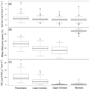
Figure 2.Plot-averaged(a)net N2O flux,(b)water-filled pore space, and(c)resin-extractable NO−₃ flux among habitats. Boxes enclose

the interquartile range, whiskers indicate the 90th and 10th percentiles. Lower case letters indicate statistically significant differences among means (Fisher’s LSD,P <0.05).

oxygen content in the 0–10 cm depth, soil temperature, air temperature, and resin-extractable inorganic N flux (NH+₄, NO−₃).

Water-filled pore space varied significantly as a func-tion of habitat, season, habitat by season, and topography (F10,304=637.96, P <0.0001; Table 3; Figs. 2b, 3;

Sup-plement Table S1b). Habitat accounted for the largest pro-portion of variance in the model (78.1 %), followed by season (0.6 %), habitat by season interaction (0.6 %), and topography (0.4 %) (Supplement Table S1b). Each habi-tat differed significantly from the others (Fisher’s LSD,

P <0.05), with the highest WFPS observed in montane

grassland (88.4±0.3 %), followed by premontane forest (51.6±1.3 %), lower montane forest (39.0±0.9 %), and up-per montane forest (35.0±1.5 %) (Fig. 2b). WFPS var-ied significantly between seasons (t test, P <0.05), with a mean dry season value of 52.1±2.4 % compared to a mean wet season value of 59.5±1.6 % (Table 3). The sig-nificant habitat by season interaction is due to the fact that some habitats showed seasonal trends in WFPS whereas oth-ers did not. Whereas lower montane and upper montane forests all showed a significant reduction in WFPS during the dry season, premontane forest and montane grasslands

showed no seasonal differences in WFPS (Table 3, Fig. 3). For topography, the main effect was that the basin landform had significantly higher WFPS than the other landforms. The basin landform showed a mean WFPS of 89.3±0.1 %, whereas WFPS in other landforms ranged from 51.7±2.2 to 57.7±2.7 %.

Soil oxygen in the 0–10 cm depth varied significantly as a function of habitat, habitat by season, and topogra-phy (F10,242=27.70,P <0.0001; Table 3; Supplement

Ta-ble S1c). Habitat accounted for the largest proportion of vari-ance in the model (66.9 % of the total varivari-ance), followed by topography (8.4 %), habitat by season (3.5 %) (Supple-ment Table S1c). For habitat, multiple comparisons tests in-dicated that only montane grasslands showed significantly lower soil O2content than the other habitats (13.5±0.6 %),

while the others showed statistically similar soil O2

val-ues to each other (18.6±0.2 to 19.5±0.1 %; Fisher’s LSD,

P <0.05). For topography, multiple comparisons tests

indi-cated that the basin landform showed statistically lower soil O2 content than the other landforms (7.4±2.3 %), whereas

the other topographic features showed statistically similar values, ranging from 16.9±0.6 to 18.2±0.2 % (Fisher’s

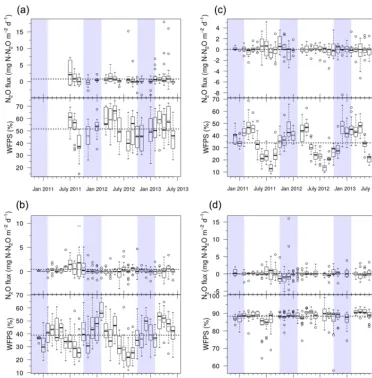
interac-Figure 3.Time series of net N2O flux and water-filled pore space (WFPS). Panels indicate data for(a)premontane forest,(b)lower montane

forest, (c)upper montane forest, and (d) montane grasslands for the 30-month study period beginning in January 2011 and ending in June 2013. The broken horizontal line running across each panel denotes the overall mean N2O flux or WFPS for that habitat. The dashed

line in each box indicate median values and the black lines indicate means. Dry and wet seasons are denoted by vertical shading on the graph, with the dry season (May to September) highlighted in white and the wet season (October to April) in light blue.

tion was due to the fact that only montane grassland showed a significant difference in O2content between wet and dry

season, whereas other habitats showed similar soil O2values

(Table 3).

For soil temperature, the effects of habitat, season, habi-tat by season, and topography were all significant (F10,292=

790.7, P <0.0001; Supplement Table S1d). Habitat ac-counted for the largest proportion of variance in the model (85.5 % of the total variance), followed by season (1.4 %), habitat by season interaction (0.5 %), and topog-raphy (0.3 %) (Supplement Table S1d). Each habitat dif-fered significantly from the others (Fisher’s LSD,P <0.05), with the highest soil temperature observed for premontane forest (20.5±0.1◦C), followed by lower montane forest (17.8±0.1◦C), upper montane forest (11.5±0.1◦C), and

montane grasslands (10.6±0.2◦C). Soil temperature var-ied significantly between season (t test, P <0.05), with a mean dry season value of 13.9±0.4◦_{C compared to a mean}

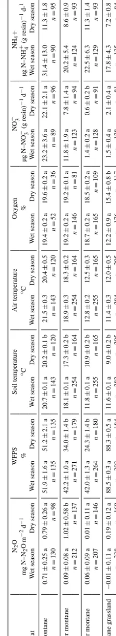
T able 3. Seasonal patterns in net N2 O flux, net inor g anic N flux, and en vironmental v ariables. Lo wer -case letters indicate dif ference among seasons within habitats ( t test on Box–Cox transformed data, P < 0.05). V alues reported here are means and standard errors. N2 O WFPS Soil temperature Air temperature Oxygen NO − 3 NH 4 + mg N–N 2 O m − 2d − 1 % ◦C ◦C % µg N–NO − 3 (g resin) − 1d − 1 µg N–NH + 4 (g resin) − 1 d-1 Habitat W et season Dry season W et season Dry season W et season Dry season W et season Dry season W et season Dry season W et season Dry season W et season Dry season Premontane 0.71 ± 0.25 a 0.79 ± 0.26 a 51.9 ± 1.6 a 51.2 ± 2.1 a 20.7 ± 0.1 a 20.2 ± 0.1 b 21.5 ± 0.3 20.4 ± 0.5 19.4 ± 0.2 a 19.6 ± 0.2 a 23.2 ± 3.6 a 22.1 ± 2.1 a 31.4 ± 13.0 11.3 ± 1.8 n = 130 n = 98 n = 135 n = 135 n = 143 n = 120 n = 143 n = 120 n = 52 n = 36 n = 89 n = 96 n = 90 n = 95 Lo wer montane 0.09 ± 0.08 a 1.02 ± 0.58 b 42.2 ± 1.0 a 34.0 ± 1.4 b 18.1 ± 0.1 a 17.3 ± 0.2 b 18.9 ± 0.3 18.3 ± 0.2 19.2 ± 0.2 a 19.2 ± 0.1 a 11.8 ± 1.9 a 7.8 ± 1.4 a 20.2 ± 5.4 8.6 ± 0.9 n = 212 n = 137 n = 271 n = 179 n = 254 n = 164 n = 254 n = 164 n = 146 n = 81 n = 123 n = 94 n = 124 n = 93 Upper montane 0.06 ± 0.09 a 0.01 ± 0.11 a 42.0 ± 1.3 a 24.3 ± 1.4 b 11.8 ± 0.1 a 10.9 ± 0.2 b 12.8 ± 0.2 12.5 ± 0.3 18.7 ± 0.2 a 18.5 ± 0.2 a 1.4 ± 0.2 a 0.6 ± 0.2 b 22.5 ± 6.3 11.3 ± 1.4 n = 207 n = 146 n = 264 n = 180 n = 255 n = 165 n = 255 n = 165 n = 165 n = 109 n = 128 n = 91 n = 129 n = 93 Montane grassland − 0.01 ± 0.11 a 0.19 ± 0.12 a 88.5 ± 0.3 a 88.3 ± 0.5 a 11.6 ± 0.1 a 9.0 ± 0.2 b 11.4 ± 0.3 12.0 ± 0.5 12.2 ± 0.9 a 15.4 ± 0.8 b 1.5 ± 0.4 a 2.1 ± 0.4 a 17.8 ± 4.3 7.2 ± 0.8 n = 238 n = 160 n = 303 n = 184 n = 282 n = 205 n = 284 n = 205 n = 176 n = 117 n = 128 n = 81 n = 135 n = 84

For air temperature, only the effect of habitat was signif-icant (F10,292=103.2, P <0.0001; Tables 3, S1e). A

mul-tiple comparisons test indicated that each habitat showed significantly different temperatures compared to the oth-ers (Fisher’s LSD, P <0.05). Premontane forest showed the highest air temperatures (21.0±0.3◦C), followed by lower montane forest (18.7±0.2◦C), upper montane for-est (12.7±0.2◦C), and montane grassland (11.7±0.3◦C). Other variables did not significantly affect air temperature.

For resin-extractable NH+₄ flux, even though the three-way ANOVA model was not statistically significant, the overall trend was towards significantly lower NH+₄ flux in the dry season (9.6±0.7 µg N–NH4g resin−1d−1)compared to the

wet season (22.3±3.6 µg N–NH4g resin−1d−1)(F10,164=

1.3, P >0.2; Tables 3, S1f).

Resin-extractable NO−₃ flux showed different patterns from NH+₄ flux, with significant effects of habitat, to-pography, and habitat by season but not of season alone (F10,164=39.0,P <0.0001; Fig. 2c; Tables 3, S1g).

Habi-tat accounted for the largest proportion of the variance (61.5 %), followed by topography (4.7 %), and habitat by season (1.9 %). Premontane forest showed the highest NO−₃ flux (22.6±2.0 µg N–NO3g resin−1d−1), followed by

lower montane forest (10.0±1.2 µg N–NO3g resin−1d−1)

(Fisher’s LSD, P <0.05; Fig. 2c). Upper montane for-est (1.1±0.2 µg N–NO3g resin−1d−1) and montane

grass-land (1.7±0.3 µg N–NO3g resin−1d−1) showed

signif-icantly lower NO−₃ flux than the other two habi-tats (Fisher’s LSD, P <0.05; Fig. 2c), with values that were not significantly different from each other (Fisher’s LSD, P >0.05; Fig. 2c). For the effect of topography, multiple comparisons tests indicated that flat landforms (12.1±1.8 µg N–NO3g resin−1d−1) and

slope landforms (10.2±1.6 µg N–NO3g resin−1d−1)

dif-fered significantly from ridge landforms (6.6±1.4 µg N– NO3g resin−1d−1) (Fisher’s LSD, P <0.05). The basin

landform (3.8±1.3 µg N–NO3g resin−1d−1), despite the

lower mean values, showed an overlapping range with the other landforms (Fisher’s LSD,P >0.05). The habitat by season interaction was due to the fact that upper mon-tane forest shows a significant seasonal fluctuation in resin-extractable NO−₃ (Fisher’s LSD, P <0.05), whereas the other habitats show no significant seasonal trend (Fisher’s

LSD,P >0.05; Table 3).

3.3 Effects of environmental variables on N2O flux For the whole dataset, the relationship between N2O flux and

indi-vidual factors were weakly but significantly correlated with N2O flux for the pooled dataset. These included soil

temper-ature (r2=0.04, P <0.0004), air temperature (r2=0.04,

P <0.0008), and resin-extractable NO−₃ flux (r2=0.03,

P <0.03). Water-filled pore space also showed a very weak

negative correlation with N2O flux at the borderline of

statis-tical significance (r2=0.01,P <0.06).

For individual habitats, we explored how variations in en-vironmental conditions influenced N2O flux using multiple

regression, with WFPS, oxygen, soil temperature, air temper-ature, resin-extractable NH+₄ flux, and resin-extractable NO−₃ flux as explanatory variables. Only the multiple regression analysis for lower montane forest showed a borderline sig-nificant result, though only at theP <0.07 level (r2=0.36). The multiple regression models for all the other habitats were not statistically significant (P >0.4). Lower montane for-est was the only habitat that showed a significant effect of season on N2O flux (Sect. 5.1), and our multiple regression

model corroborated this result by showing that seasonal fluc-tuations in air temperature, soil temperature, WFPS (Fig. 3b), and NH+₄ all correlated with N2O flux (P <0.05). Air

tem-perature explained the largest proportion of variance in the data (26.2 %; negative trend), followed by soil temperature (15.5 %; positive trend), WFPS (13.7 %; negative trend), and resin-extractable NH+₄ flux (11.6 %; negative trend).

3.4 Water-filled pore space manipulation

15_N–N

2O and 15N–N2 fluxes showed a biphasic response

(Limmer and Steele, 1982), with significantly different flux rates in the first 24 h of incubation compared to the later pe-riod of incubation (i.e. 24–48 h). Flux of15N–N2O, and15N–

N2, were therefore divided into early (0–24 h) and late (24–

48 h) phase flux.

3.4.1 Role of nitrification and nitrate reduction in N2O production

The15N flux data indicate that nitrate reduction (i.e. denitri-fication) was the dominant source of N2O from these soils,

while nitrification was only a minor contributor to15N–N2O

production (Supplement Fig. S1). The15N–N2O and15N–N2

fluxes were analysed using a full factorial ANOVA on Box– Cox transformed data with habitat, moisture level, form of

15_{N-label added (i.e.}15_NH15

4 NO3 or 14NH 15

4 NO3),

incuba-tion phase, and all their interacincuba-tion terms as independent vari-ables. Notably, this analysis revealed that the form of15N la-bel added (i.e.15N–NH15₄ N–NO3or14N–NH15₄ N–NO3)did

not significantly alter15N–N2O flux, indicating that

produc-tion of 15N–N2O from nitrification was weak to negligible

(Supplement Fig. S1). In order to simplify our statistical analyses, all subsequent analyses were performed using only habitat, moisture level, incubation phase, and their interac-tion terms as independent variables. For these tests, which are described below, the “total” flux of15N–N2O or15N–N2

represents gas produced by both nitrification and nitrate re-duction.

3.4.2 15N–N2O flux

For the total 15N–N2O flux data, we used a full

fac-torial ANOVA on Box–Cox transformed data with habi-tat, moisture level, incubation phase, and all their inter-actions as independent variables. We found that moisture level, habitat by incubation phase, and habitat by mois-ture by incubation phase were significantly related to15N– N2O flux (ANOVA, F31,321=3.06, P <0.0001; Fig. 4;

Supplement Table S2a). Of the three main factors (i.e. habitat, moisture level, incubation phase), moisture level was the dominant control on 15N–N2O flux (Supplement

Table S2a). The highest 15N–N2O flux was observed in

the 90 % WFPS (42±9 ng N2O–15N g−1d−1) and 50 %

WFPS (29±10 ng N2O–15N g−1d−1) treatments, and the

lowest flux in the 30 % (3±1 ng N2O–15N g−1 d−1) and

70 % (7±2 ng N2O–15N g−1d−1)treatments (Fisher’s LSD,

P <0.05; Fig. 4). The habitat by incubation phase

interac-tion indicated that some habitats showed different flux rates during early and late phases of the incubation (Fig. 4). Pre-montane and lower Pre-montane forest showed statistically sim-ilar15N–N2O flux during early and late incubation phases.

Upper montane forest mineral layer soils showed a signifi-cant increase in15N–N2O flux from early to late incubation

phases (5±2 ng N2O–15N g−1d−1 versus 42±13 ng N2O– 15_{N g}−1_d−_{1; t test, P <0.003), while montane grasslands}

showed a significant decrease in15N–N2O flux from early to

late incubation phases (60±23 ng N2O–15N g−1d−1versus

6±9 ng N2O–15N g−1d−1, respectively; t test, P <0.02).

The habitat by moisture by incubation phase effect stems from complex and varying responses of soils from different habitats to differences in moisture level and incubation phase (Fig. 4).

3.5 15N–N2flux

For the total 15N–N2 flux data, we used a full factorial

ANOVA on Box–Cox transformed data with habitat, mois-ture level, incubation phase, and all their interactions as independent variables. We found that all of the main fac-tors and their interaction terms were statistically signif-icant (ANOVA, F31,317=14.20, P <0.0001; Supplement

Table S2b). Of the three main factors, habitat was the dominant control on15N–N2flux (Supplement Table S2b).

Lower montane forest showed the highest 15N–N2 flux

(694±83 ng N2–15N g−1d−1); premontane forest and upper

montane forest mineral layer soil showed intermediate levels of flux (326±53 and 171±20 ng N2–15N g−1d−1,

respec-tively); and montane grassland soil showed the lowest flux (123±23 ng N2O–15N g−1d−1) (Fisher’s LSD, P <0.05;

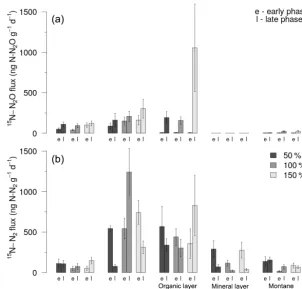
treat-Figure 4.Total(a)15N–N2O flux and(b)15N–N2flux during the early (≤24 h) and late (>24 h) incubation phases of the water-filled pore

space (WFPS) experiment. Results from the 90 % WFPS treatment are shown in dark grey, while data from the 70, 50, and 30 % WFPS treatments are shown in mid grey, light grey, and white, respectively. The bar charts show means and standard errors.

ment having significantly higher flux than the other treat-ments (90 % WFPS treatment: 437±77 ng N2–15N g−1d−1;

pooled average for all other treatments: 294±28 ng N2– 15_{N g}−1_d−1_{) (Fisher’s LSD, P <0.05). Incubation phase}

was the least important control on15N–N2flux, with slightly

greater flux of 15N–N2 during the late compared to the

early phase of the incubations (373±44 ng N2–15N g−1d−1

versus 288±37 ng N2–15N g−1d−1)(t test,P <0.07). The

habitat by moisture level interaction indicates that flux from different habitats showed varying moisture responses (Fig. 4). For example, 15N–N2 flux from premontane

for-est and upper montane forfor-est mineral layer soil showed no responses to moisture. In contrast, for lower mon-tane forest, flux was greatest for the 90 % WFPS treat-ment (1365±201 ng N2–15N g−1d−1), lowest for the 70 %

WFPS treatment (257±128 ng N2–15N g−1d−1), and at

in-termediate levels for the 30 % and 50 % WFPS treatments (664±131 and 492±79 ng N2–15N g−1d−1, respectively)

(Fisher’s LSD, P <0.05). The pattern for montane grass-land was different again; here, only the 90 % WFPS treat-ment showed significantly greater flux (171±32 ng N2– 15_{N g}−1_d−1_{)compared to the other treatments (pooled}

av-erage: 105±29 ng N2–15N g−1d−1) (Fisher’s LSD, P <

0.05).

3.5.1 N2O yield

For the N2O yield, we used a full factorial ANOVA on Box–

Cox transformed data with habitat, moisture level, incuba-tion phase, and all their interacincuba-tions as independent variables. We found that habitat, moisture level, habitat by moisture level, habitat by phase, and habitat by moisture level by phase significantly influenced N2O yield (ANOVA,F31,313=9.85,

P <0.0001; Supplement Table S2c). Of the three main

fac-tors, habitat was the best predictor of N2O yield

(Supple-ment Table S2c). N2O yield was highest for the montane

grassland (0.61±0.06), lowest for lower montane forest (0.19±0.04), while premontane forest and upper montane forest mineral layer soil showed similar intermediate values (0.40±0.05 and 0.42±0.05, respectively) (Fisher’s LSD,

P <0.05). Moisture level explained much less of the

vari-ance in the dataset (Supplement Table S2c); N2O yield was

highest for the 70 % WFPS treatment (0.51±0.06), while the 30, 50 and 90 % WFPS treatments showed statistically simi-lar values (0.35±0.05, 0.39±0.05, and 0.36±0.05, respec-tively) (Fisher’s LSD,P <0.05). For the habitat by moisture level interaction, this reflects the fact that only lower montane forest and upper montane forest showed differences in N2O

forest, N2O yield was greatest in the 70 % WFPS treatment

(0.51±0.11), whereas the other treatments were not statisti-cally different from each other (pooled average: 0.09±0.03) (Fisher’s LSD, P <0.05). Upper montane forest mineral layer soil showed the highest N2O yield for the 90 %

treat-ment (0.72±0.08), lowest yield for the 30 % WFPS treat-ment (0.20±0.09), and intermediate N2O yields for the 50

and 70 % WFPS treatments (0.29±0.09 and 0.50±0.11, respectively) (Fisher’s LSD, P <0.05). For the habitat by incubation phase interaction, this reflects the fact that up-per montane forest mineral layer soil showed an increase in N2O yield from early to late phase, while montane grassland

showed a decrease in N2O yield from early to late phase.

The habitat by moisture level by incubation phase interac-tion reflects the complex and varied responses of soils from different habitats to changes in moisture level and incubation phase (Fig. 4).

3.6 Litter manipulation experiment

In order to investigate the relationship between leaf litter in-put rates and N2O flux, we used a Generalized Linear Model

(GLM) and an ANCOVA that included habitat, litter treat-ment, season, WFPS, litter input rate, litter C input rate, litter N input rate, soil temperature and air temperature as independent variables. The analysis was also repeated us-ing ANCOVA on Box–Cox transformed data. Both analyses revealed no significant statistical relationship between N2O

flux and any of these environmental variables, with the ex-ception of soil temperature, which showed only a weak pos-itive relationship to N2O flux when the data was analysed

using the GLM (P <0.05). This relationship was not de-tected using ANCOVA. Bivariate regression of soil tempera-ture against N2O flux indicated that the relationship was

rel-atively weak, withr2=0.01 (P <0.05). 3.7 Nitrate addition experiment

15_N–N

2O and 15N–N2 fluxes showed a biphasic response

(Limmer and Steele, 1982), with significantly different flux rates in the first 24 h of incubation compared to the later pe-riod of incubation (i.e. 24–48 h). Flux of15N–N2O, and15N–

N2, were therefore divided into early (0–24 h) and late (24–

48 h) phase flux. 3.7.1 15N–N2O flux

For the15N–N2O flux data, we used a full factorial ANOVA

on Box–Cox transformed data with habitat, N addition level, incubation phase, and all their interaction terms as inde-pendent variables. Habitat, incubation phase, and the habi-tat by incubation phase interaction all significantly influ-enced15N–N2O flux (ANOVA,F29,149=5.67,P <0.0001;

Fig. 5; Supplement Table S3a). Notably, N addition level did not significantly influence 15N–N2O flux. Of the three

main factors (i.e. habitat, N addition level, incubation

phase), habitat was the best predictor of 15N–N2O flux,

explaining the largest proportion of the variance (Supple-ment Table S3a). Upper montane forest organic layer soils showed the highest flux (238±160 ng N2O–15N g−1d−1),

lower montane (179±48 ng N2O–15N g−1d−1) and

pre-montane (86±16 ng N2O–15N g−1d−1) forest showed

in-termediate flux, while montane grasslands (11±4 ng N2O– 15_{N g}−1_d−1_{)and upper montane forest mineral layer soils}

(0.06±0.01 ng N2O–15N g−1d−1) showed the lowest flux

(Fisher’s LSD,P <0.05). The effect of incubation phase was attributable to significantly greater15N–N2O flux during the

late compared to early incubation phases (164±66 ng N2O– 15_{N g}−1_d−1 _{versus 42±11 ng N}

2O–15N g−1d−1; t test,

P <0.05; Fig. 5). The habitat by incubation phase

interac-tion was caused by some habitats showing higher flux in cer-tain incubation phases than others (Fig. 5). During the early phase, lower montane and premontane forests collectively showed the highest flux (Fig. 5; Fisher’s LSD,P <0.05). In contrast, during the late incubation phase, upper montane for-est organic layer soils, lower montane forfor-est, and premontane forest now showed the highest flux (Fig. 5; Fisher’s LSD,

P <0.05).

3.7.2 15_N–N 2flux

For the15N–N2flux data, we used a full factorial ANOVA

on Box–Cox transformed data with habitat, N addition level, incubation phase, and all their interaction terms as independent variables. Only habitat significantly influenced flux, while other terms were not significant (ANOVA,

F29,149=1.66, P <0.05; Fig. 5; Supplement Table S3b).

Lower montane and upper montane forest organic layer soils showed the highest flux (472±139 and 576±117 ng N2– 15_{N g}−1_d−1_{, respectively), while all other habitats showed}

similar flux rates (105±19 ng N2–15N g−1d−1) (Fisher’s

LSD,P <0.05; Fig. 5).

3.7.3 N2O yield

For the N2O yield, we used a full factorial ANOVA on Box–

Cox transformed data with habitat, N addition level, incu-bation phase (i.e. early versus late), and all their interac-tion terms as independent variables. We found that none of these factors predicted N2O yield (ANOVA,F29,149=0.75,

P >0.82; Supplement Table S3c). The overall mean N2O

yield for the pooled dataset was 0.53±0.04.

4 Discussion

4.1 Effects of seasonality and soil moisture on N2O flux Nitrous oxide flux in the Kosñipata Valley showed weak sea-sonality, with greater N2O flux during the dry season

Figure 5. (a)15N–N2O flux and(b)15N–N2flux during the early (≤24 h) and late (>24 h) incubation phases of the NO−₃ addition

exper-iment. Results from the+50 % NO−₃ addition are shown in dark grey, while data from the+100 and+150 % treatments are shown in mid grey and light grey, respectively. The bar charts show means and standard errors.

by strong seasonality in N2O flux from lower montane

for-est (Teh et al., 2014). In contrast, other habitats showed little or no seasonal variation in N2O flux. This weak

seasonal-ity in N2O flux across the Kosñipata Valley probably stems

from relatively modest variation in environmental variables among seasons (Table 3), in accordance with observations from elsewhere in the Andes (Baldos et al., 2015; Müller et al., 2015; Wolf et al., 2011). For example, while soil mois-ture (i.e. WFPS) varied significantly between seasons in the dataset as a whole, the absolute difference in WFPS between dry season and wet season were relatively small (i.e. 7.4 %). Indeed, some habitats showed much smaller variations in soil moisture, such as premontane forest and montane grassland that showed no significant seasonal variation in WFPS what-soever (Table 3).

One critical factor contributing to these weak seasonal trends in N2O flux is the atypical response of N2O flux to

changes in soil moisture. Nitrous oxide flux showed a weak but negative correlation with WFPS in the field dataset (r2=

0.01,P <0.06 for the pooled dataset), rather than following

a curvilinear pattern predicted by denitrification theory (Fire-stone and Davidson, 1989; Fire(Fire-stone et al., 1980; Weier et al., 1993; Davidson, 1991). Likewise, in our soil moisture ma-nipulation experiments, nitrification made a minor contribu-tion to N2O production, irrespective of soil moisture content

(Supplement Fig. S1). This finding is contrary to theoretical predictions of N2O production by ammonia-oxidizing

bacte-ria (AOB), where N2O production from ammonia oxidation

is thought to make an important contribution to N2O flux

at lower soil moisture contents (i.e. 30–60 % WFPS) (Fire-stone and Davidson, 1989; Fire(Fire-stone et al., 1980; Weier et al., 1993; Davidson, 1991). At higher soil moisture contents (i.e.>60 % WFPS), N2O flux showed a non-linear response

to increasing WFPS, with two distinct peaks in N2O flux at

90 and 50 % WFPS (Fig. 4). Collectively, these findings sug-gest that the role of soil moisture in regulating N2O flux is

more complex than predicted by existing theory, falsifying our first two hypotheses.

What could explain these unexpected trends? We believe that these patterns occurred due to the complex interplay be-tween environmental conditions and the microbial processes that produce N2O in soil (i.e. ammonia oxidation by

ar-chaea, ammonia oxidation by bacteria, denitrification, dis-similatory nitrate reduction to ammonium). We suspect that the action of lesser-known microbial processes, such as ox-idation of ammonia by archaea and dissimilatory nitrate re-duction to ammonium (DNRA), may explain the divergence from theoretical norms. Our expectations of how N2O

exclusively by AOB and denitrifying bacteria, with the for-mer operating at lower soil moisture content (i.e. 30–60 % WFPS) and the latter at higher soil moisture content (i.e.

>60 % WFPS) (Firestone and Davidson, 1989; Firestone et al., 1980; Weier et al., 1993; Davidson, 1991). More recent advances in soil N research, however, have highlighted the importance of other microbial taxa or processes, not previ-ously considered in conceptual or process-based models. For example, recent work in acidic soils have demonstrated that ammonia oxidizing archaea (AOA) play a more important role than AOB in ammonia oxidation, but produce signifi-cantly less N2O due to differences in metabolism (Hink et

al., 2016; Prosser and Nicol, 2008). Likewise, under higher soil moisture conditions (>60 % WFPS), DNRA – a pro-cess that produces substantially less N2O than denitrification

and which also competes for NO−₃ with denitrification – can dominate nitrate reduction, depending on redox conditions and the relative availability of labile C and N (Morley and Baggs, 2010; Pett-Ridge and Firestone, 2005; Silver et al., 2001; Baldos et al., 2015; Müller et al., 2015). Thus, given the low pH of the soils in Kosñipata Valley (Table 1), it is likely that AOA dominate ammonia oxidation at lower levels of soil moisture, explaining the negligible amounts of N2O

produced from nitrification in the 30 and 50 % WFPS treat-ments. As soils become wetter, the non-linear response of N2O flux to increasing soil moisture may reflect

competi-tion for substrates (e.g. NO−₃, reducing equivalents) between DNRA and denitrification (Morley and Baggs, 2010; Silver et al., 2001), or may indicate that DNRA is making a larger contribution to N2O flux than denitrification (Streminska et

al., 2012).

These findings are important and noteworthy, given that climatically driven variations in soil moisture content are thought to be one of the dominant drivers for N2O flux in

the seasonally dry tropics (Davidson, 1991; Firestone and Davidson, 1989; Groffman et al., 2009; Davidson and Ver-chot, 2000; Teh et al., 2014; van Lent et al., 2015; Werner et al., 2007). Moreover, similar results from comparable re-search sites in the Ecuadorian Andes lend credence to our claims (Baldos et al., 2015; Müller et al., 2015). For example, Müller et al. (2015) found that nitrification produced little or no N2O in acidic Ecuadorian soils, in agreement with

find-ings from this study. Likewise,15N isotope pool dilution ex-periments, in comparable habitats and elevations to our own, revealed that DNRA played a significant role in nitrate reduc-tion, supporting the notion that DNRA may represent a sub-stantial sink for NO−₃ in Peruvian soils (Baldos et al., 2015; Müller et al., 2015). Existing process-based models, which are used to construct bottom–up emissions inventories for the tropics (Werner et al., 2007), often assume that N2O is

de-rived primarily from AOB and denitrification, with moisture response curves based on existing theoretical relationships (Li et al., 2000; Werner et al., 2007; Smith et al., 2007). How-ever, if these more “normative” soil moisture response curves are inapplicable to montane tropical ecosystems, due to the

activity of AOA and DNRA, then a re-conceptualization of the soil moisture–N2O flux relationship may be required.

Moreover, if weak seasonality or aseasonality in N2O flux

is the norm in Andean ecosystems (Müller et al., 2015; Wolf et al., 2011), then this finding may have wider implications for understanding spatial or temporal trends in regional at-mospheric budgets (Kort et al., 2011; Nevison et al., 2004, 2007; Saikawa et al., 2014).

4.2 Role of substrate limitation in regulating N2O flux In accordance with our earlier work (Teh et al., 2014) and re-search conducted in analogous ecosystems in Ecuador (Bal-dos et al., 2015; Müller et al., 2015; Wolf et al., 2011), we found strong evidence that N2O flux was constrained by the

availability of NO−₃, partially supporting our third hypoth-esis. In contrast, N2O flux was unresponsive to short-term

changes in labile organic matter (i.e. leaf litter-fall) inputs, indicating that N2O flux and nitrate reduction were not C

lim-ited. This latter result is significant for modelling and extrap-olating N2O flux from these habitats, because many

process-based models assume that N cycling and turnover of labile or-ganic matter are intimately linked through processes such as litter production and decomposition (Li et al., 2000; Werner et al., 2007; Smith et al., 2007).

Evidence for NO−₃ limitation of N2O flux comes from both

our field and laboratory data, and suggests that “habitat” may be a good proxy for NO−₃ availability and N2O flux because

these two variables co-vary with habitat. For example, we observed an inverse trend in field N2O flux, with

premon-tane forest showing significantly greater flux than the other habitats’ elevation (Table 3, Fig. 2a). This inverse trend was also reflected in the resin-extractable NO−₃ flux measured in the field and the15N–N2O flux measured in the NO−₃

ad-dition experiment in the laboratory (Figs. 2c, 5a). Further-more, the behaviour of the15N–NO−₃ amended soils during the early (≤24 h) and late (>24 h) phases of the incubation experiment suggests that soils from more N-poor habitats (i.e. those with lower rates of resin-extractable NO−₃ flux; Table 3, Fig. 2c) showed a greater proportional increase in

15_N–N

2O flux following NO−3 addition than N-rich habitats

(i.e. those with higher rates of resin-extractable NO−₃ flux; Table 3, Fig. 2c), suggesting that15N–N2O flux was more

NO−₃ limited in N-poor soils (Fig. 5). Soils from the upper montane forest organic layer, montane grasslands, and upper montane forest mineral layer showed the lowest 15N–N2O

flux during the early phase of soil incubation, but the great-est proportional increase in flux during the late phase of soil incubation, rising by factors of 59, 5, and 2, respectively. In contrast, lower montane and premontane forest soils showed the smallest proportional increase in the late phase of soil incubation (i.e. 1.7 times increase). Last, the relatively low N2O yield observed in our soil moisture manipulations is

thought to be broadly indicative of low NO−₃ conditions (i.e.

notion that N2O flux in this region is generally NO−₃ limited

(Schlesinger, 2009; Fang et al., 2015; Weier et al., 1993). Interestingly, increasing NO−₃ availability per se did not stimulate15N–N2O flux and15N–N2flux, or alter N2O yield

during the early phase (<24 h) of the NO−₃ addition exper-iment, even though we did observe that 15N–N2O flux

in-creased during the late phase (>24 h) of the experiments (please see Fig. 5 and the discussion in the preceding para-graph). Rather, ANCOVA suggests that15N–N2O and15N–

N2fluxes in the early phase of the NO−3 addition experiment

were better predicted by habitat, i.e. that soil provenance was a better predictor of 15N–N2O flux than N treatment.

N2O yield, normally a sensitive indicator of NO−₃

availabil-ity (Blackmer and Bremner, 1978; Weier et al., 1993; Par-ton et al., 1996), also showed no immediate response to the amount of 15N–NO−₃ added, nor any of the other ex-planatory variables. One explanation for this, consistent with the notion that N2O flux is NO−₃ limited, is that

nitrate-reducing microbes in these soils may have a relatively low half-saturation constant (Km)for NO−₃, and effectively

uti-lize NO−₃ whenever concentrations increase above baseline (i.e. non-limiting) levels (Holtan-Hartwig et al., 2000). As a consequence, we may be unable to differentiate among NO−₃ treatments in the early phase of the experiment, because the amount of NO−₃ added exceeded theKmfor these soils. This

finding is also in agreement with results from long-term N fertilization studies, which suggest that substantive shifts in N2O flux are only likely to occur after prolonged exposure to

high levels of N (i.e.>1 year), rather than due to transient fluctuations in N availability (Baldos et al., 2015; Corre et al., 2010; Müller et al., 2015; Hall and Matson, 1999; Koehler et al., 2012).

4.3 Implications for annual atmospheric budgets and gaseous N loss

Montane ecosystems in the Kosñipata Valley were net sources of atmospheric N2O, affirming our prior results (Teh

et al., 2014). The flux for this multi-annual dataset was com-parable to the preliminary values reported in our earlier pub-lication, with an unweighted mean flux of 0.27±0.07 mg N– N2O m−2d−1 observed over a 30-month period compared

to 0.22±0.12 mg N–N2O m−2d−1 recorded over a

13-month period (Teh et al., 2014). These values correspond to unweighted mean annual fluxes of 0.99±0.26 kg N2O–

N ha−1yr−1 and 0.80±0.44 kg N2O–N ha−1yr−1,

respec-tively. However, in order to derive more accurate estimates of the annual contribution of the Kosñipata Valley to the re-gional atmospheric budget of N2O, it is necessary to account

for differences in land area for different habitats and varia-tion in the magnitude of N2O flux between seasons. Thus,

we conducted a simple weighted upscaling exercise to more fully account for these two sources of variation (Table 4). Using the N2O yield data from the laboratory tracer

experi-ments, we also estimated the annual N2flux and total gaseous _Table