Generation and validation of spatial distribution of hourly wind speed time-series using machine learning

(1)

Veronesi, F. and Grassi, S. 2018. Generation and validation of spatial distribution of hourly wind speed time‐series using machine learning. Journal of Physics: Conference Series, 749 (012001).

Generation and validation of spatial

distribution of hourly wind speed

time-series using machine learning

by Veronesi, F. and Grassi, S.

Copyright, Publisher and Additional Information: Publishers version distributed under the terms of the Creative Commons Attribution Licens

e:

https://creativecommons.org/licenses/by/3.0/

DOI:

10.1088/1742-6596/749/1/012001

(2)

Journal of Physics: Conference Series

PAPER • OPEN ACCESS

Generation and Validation of Spatial Distribution of Hourly Wind Speed

Time-Series using Machine Learning

To cite this article: F Veronesi and S Grassi 2016 J. Phys.: Conf. Ser. 749 012001

View the article online for updates and enhancements.

(3)

Generation and Validation of Spatial Distribution of

Hourly Wind Speed Time-Series using Machine

Learning

F Veronesi & S Grassi

Institute of Cartography and Geoinformation – ETH Zurich Stefano-Franscini-Platz 5, 8093 Zurich

[email protected]

Abstract. Wind resource assessment is a key aspect of wind farm planning since it allows to estimate the long term electricity production. Moreover, wind speed time-series at high resolution are helpful to estimate the temporal changes of the electricity generation and indispensable to design stand-alone systems, which are affected by the mismatch of supply and demand. In this work, we present a new generalized statistical methodology to generate the spatial distribution of wind speed time-series, using Switzerland as a case study. This research is based upon a machine learning model and demonstrates that statistical wind resource assessment can successfully be used for estimating wind speed time-series. In fact, this method is able to obtain reliable wind speed estimates and propagate all the sources of uncertainty (from the measurements to the mapping process) in an efficient way, i.e. minimizing computational time and load. This allows not only an accurate estimation, but the creation of precise confidence intervals to map the stochasticity of the wind resource for a particular site. The validation shows that machine learning can minimize the bias of the wind speed hourly estimates. Moreover, for each mapped location this method delivers not only the mean wind speed, but also its confidence interval, which are crucial data for planners.

Keywords: wind resource assessment, time-series, confidence intervals.

1. Introduction

Wind resource assessment is a key component of the planning phase for every wind farm project. In particular, wind speed time-series at fine resolution (i.e. hourly or sub-hourly) are helpful to estimate the temporal changes of the electricity generation and indispensable to design stand-alone systems that are affected by the mismatch of supply and demand. In addition, the variability of wind speed is important to evaluate the impact of the electricity injection into the power grid. Wind speed and direction data are measured worldwide by weather stations at various time-intervals. However, their coverage is inadequate to identify suitable locations to build new wind farms. In many cases, after a potential site has been identified, the planning phase continues with at least a year of continue wind measurements using a meteorological mast [1], which is a device that measures wind at various heights. This step highly increases the total cost of the project and therefore has a non-negligible impact on the rate of return of the initial investment. One way to decrease the planning costs is by employing techniques to estimate the temporal variability of the wind resource on the potential site, i.e. wind resource assessment.

WindEurope Summit 2016 IOP Publishing

Journal of Physics: Conference Series749(2016) 012001 doi:10.1088/1742-6596/749/1/012001

Content from this work may be used under the terms of theCreative Commons Attribution 3.0 licence. Any further distribution of this work must maintain attribution to the author(s) and the title of the work, journal citation and DOI.

(4)

Several techniques have been developed over the years to estimate the spatio-temporal pattern of the wind resource. The majority of these techniques are part of a set referred to as numerical wind flow models, which estimate the wind resource solving the physical equations that govern the motion of air in the atmosphere [2]. These methods have varying level of complexity, derived by the type and amount of equations they include. The simplest ones are the mass-consistent models [3], first developed in the 1970s, which only solve the equation of conservation of mass. On the other end of the complexity spectrum are numerical weather prediction models (NWP; [2]), which solve all the computational fluid-dynamics equations plus others that govern the energy exchanges between soil and atmosphere. These methods are able to estimate both the long term wind resource and its time variability, even though they tend to be time-consuming and computationally expensive [4].

Another branch of research has been dedicated to the development of techniques for wind resource assessment based purely on statistical algorithms. Statistical models correlate wind speed data from weather stations, with remotely sensed physical parameters, to infer the wind spatio-temporal pattern. As demonstrated in previous work [4], statistical methods are accurate, computationally efficient, and less time-consuming than physical models. These methods have been tested in the literature for estimating both the long term pattern of the wind resource (e.g. [4]–[8]) and for time-series estimations with models such as ARMA (Auto Regressive Moving-Average; [9], [10]), Markov chain [11] and autoregressive models [12]. However, the spatio-temporal prediction, i.e. the estimation of the hourly wind speed pattern in areas where no direct observations are available, of wind speed time-series using machine learning techniques is a recent research topic [13]. The major problem in wind resource assessment is the large amount of uncertainty involved, which ranges from malfunctions of the weather stations to the extrapolation of the wind speed profile in complex terrains. Assessing this uncertainty is difficult with numerical wind flow models, but straightforward with statistical wind resource assessment, which can precisely account for all these sources of uncertainties [8].

In this work, we present a new generalized statistical methodology, based on machine learning, to generate the spatial distribution of wind speed time-series, using Switzerland as a case study. This research is a continuation of the work we presented at EWEA 2015 [14], and demonstrates that statistical wind resource assessment can be successfully used for estimating wind speed time-series. In fact, this method is able to efficiently obtain reliable wind speed estimates and to propagate all the sources of uncertainty, from the measurements to the mapping process, so that the final confidence intervals allow a reliable estimation of the stochasticity of the wind resource for a particular site.

Fig. 1: Location of the automatic weather stations (red triangle) belonging to the MeteoSwiss network.

(5)

2. Materials and Methods

2.1. Dataset

We collected 10 min average wind speed data over 5 years from 161 stations of the MeteoSwiss (Swiss Federal Office of Meteorology and Climatology) network. The stations are sparsely located across Switzerland (the exact location is depicted in Fig.1) and measure wind at a height of 10 m AGL These data provide the variable for the machine learning model to estimate it in locations where no weather observations are available.

The wind speed measurements were correlated with around 8’000 predictors, consisting of environmental and climate data with different time and spatial resolutions covering Switzerland. A detailed list of all the data employed for this study, which were collected from various open data repositories, is presented in Table 1.

2.2. Machine Learning Approach

This research employed the wind resource assessment method, based on machine learning, developed by Veronesi et al. [4] to estimate the long term wind speed and direction distributions over large regions. Machine learning algorithms are very flexible since they are data driven, meaning that the method works the same way with wind long term averages or hourly observations. In this research we employed the method developed in [4] to estimate wind hourly speeds, thus the machine learning algorithm was run for a total of 8’790 times, one for each hour of the year, to provide detailed wind speed time-series.

This approach was developed to statistically estimate the wind field not only in space but also in time. In the paper we presented last year at the EWEA annual event [14], we used this approach to estimate the long term wind speed distribution in Switzerland over a 1 Km grid. With this research we went one step further, adding a temporal component to the analysis. In this work the machine learning algorithm was employed to estimate a long term hourly time-series for each grid cell. For long term time series, we mean that the 10 min data were aggregated over the entire sampling period to produce average time-series, with uncertainty, which include the range of variation of wind speed for every hour of the year. In other words, the results we present can be used to assess the average hourly range of variation of the wind resource.

One of the main objective of this study was to provide planners with more informative wind speed time-series, compared with other wind resource assessment methods. The crucial difference between statistical and physical wind resource assessments is in the way they handle uncertainty. Machine learning is perfectly able to assess its own accuracy, thus providing planners with high-resolution error information that physical methods cannot provide. This is true for long term planning, as demonstrated by Veronesi et al. [4], but it is also important in time-series analysis. Having access to a detailed uncertainty estimation may in fact allow for a more precise estimation of the risk involved in developing a site, with a finer spatio-temporal granularity compared to long term averages.

To reach this objective we devised the method in such a way as to include every possible source of uncertainty, from the variability present in the data to the error that affects the machine learning estimations. The latter is relatively easy to include, since contrary to numerical wind flow models, statistical methods are by default able to assess their uncertainty. On the contrary, the variability in the weather observations is more difficult to incorporate in the model. For example, in the 5 years of data we gathered for this experiment it is safe to assume that in certain hours the anemometers would record higher than average wind speed, maybe caused by storms. Therefore, when the 10 min data are aggregated some of them will present high values, and other low values. Using only the average speed for each hour means losing the information in regards to the variability in the data. It is important for planners to know that certain hours present historically more variable speeds, while others generally present calmer winds. For this reason, and to account for the data variability, we used a resampling approach called Bootstrapping [15] to fit multiple statistical models to the 30 hourly observations (i.e. 6 samples/hour over 5 years). This way we were able to propagate the variability from the anemometer data to the wind speed predictions, while also accounting for all other sources of uncertainty. This allowed us to provide a full uncertainty estimation, in terms of confidence intervals, for each location and each time frame we estimated.

(6)

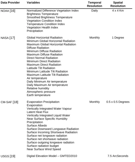
Table 1: List of global data used as predictors for the machine learning algorithm to estimate hourly wind speed in Switzerland

Data Provider Variables Temporal Resolution

Spatial Resolution

NOAA

[16]

Normalized Difference Vegetation Index Brightness Temperature

Smoothed Brightness Temperature Vegetation Condition Index

Temperature Condition Index Vegetation Health Index Precipitation

Daily 4 x 4 Km

NASA

[17]

Global Horizontal Radiation

Minimum Global Horizontal Radiation Maximum Global Horizontal Radiation Diffuse Radiation

Minimum Diffuse Radiation Maximum Diffuse Radiation Direct Normal Radiation Minimum Direct Radiation Maximum Direct Radiation Latitude Tilt Radiation

Minimum Latitude Tilt Radiation Maximum Latitude Tilt Radiation Air temperature

Daily Minimum Air temperature Daily Maximum Air temperature Relative humidity

Atmospheric pressure Earth temperature

Monthly 1 Degree

CM-SAF

[18]

Evaporation Precipitation Evaporation

Vertically Integrated Water Vapour Latent Heat Flux

Vertically Integrated Liquid Water Near Surface Specific Humidity Precipitation

Surface Albedo

Surface Downward Longwave Radiation Surface Incoming Shortwave Radiation Surface net longwave radiation

Surface net shortwave radiation Surface outgoing longwave radiation Surface radiation budget

Near Surface Wind Speed

Monthly 0.5 x 0.5 Degrees

USGS

[19]

Digital Elevation Model – GMTED2010 7.5 ArcSeconds

2.3. Validation

The validation of the estimates was carried out with a five-fold spatio-temporal cross-validation. We created a cross-validation loop consisting of 1’000 iterations. For each iteration, 20% of the weather stations were randomly excluded from the training process of the machine learning algorithm. The algorithm was then trained using data from one particular hour of the year, chosen randomly. Then the testing was done comparing the estimates from the machine learning algorithm with the wind observation from the same hour in the stations excluded from training.

(7)

The bias, i.e. the difference between wind observations and machine learning estimates, was calculated after each iteration of the validation loop. The results were then aggregated by month, to show the monthly accuracy of the spatio-temporal wind speed model. Instead of just presenting the average bias, which is not much informative, we included its full distribution as monthly box-plots.

2.4. Extrapolation to Hub Height

For extrapolating the wind speed from 10 m, i.e. the height of the weather stations, to hub height, we employed the process presented in Grassi et al. [20], briefly described here.

This process exploits the logarithmic relation between wind speed and terrain roughness indicated by Equation 1 from [21]:

𝑣̅𝐻= 𝑣̅𝑟𝑒𝑓∙

𝑙𝑛(𝐻 𝑧⁄ )𝑜

𝑙𝑛(𝐻𝑟𝑒𝑓⁄ )𝑧0

(1)

Where 𝑣̅𝐻 is the wind speed at hub height (m/s), 𝑣̅𝑟𝑒𝑓 is the wind speed at reference height (m/s), in this case 10 m, 𝐻 is the hub height (m), 𝐻𝑟𝑒𝑓 is the reference height (m), i.e. 10 m. The important parameter of this equation is 𝑧0, the roughness height. This is the parameter that controls the increase in wind speed with altitude and depends on terrain and land-use. Essentially, this parameter described the changes in the vertical wind shear caused by the friction with the earth surface, which depends directly upon the type of land cover. On areas of bare land or small vegetation, this parameter is close to zero, whereas in areas of taller vegetation or covered by buildings this parameter is closer to 1.

Equation 1 represents a standard method to extrapolate wind speed with elevation, but its accuracy is strongly dependent upon the precision of the roughness parameter. This is generally taken from literature and assigned based on the land-use and vegetation types of the location of the planned wind farm. However, this approach has some limitations, since it considers the wind shear as something that depends only on local terrain conditions and land cover. On the contrary, the downwind terrain conditions have also a large impact on the wind shear in the area considered for the turbine placement. For example, imagine we want to build a wind farm on arable land, which on its South-East side is bordered by a forest. The wind coming from this direction would have a much lower speed compared to the one coming from other directions. If we only consider the land cover of the wind farm area, i.e. arable, we will overlook this aspect, thus potentially overestimating the electricity production of the wind farm.

In Grassi et al.

[20]

the authors present an approach carried out on GIS applications that is perfectly able to take the directionality of the wind into account for computing the roughness height. This approach not only considers the terrain roughness of the local area under investigation, but also the downwind areas and their terrain conditions in respect to 12 wind directions. This approach allows a more accurate computation of the 𝑧0 factor and thus a better understanding of the potential of a site to become suitable for wind farm planning.

3. Results and Discussions

This research presents the results of a case study carried out in Switzerland to test a method, based on statistical wind resource assessment, to map the spatio-temporal pattern of wind speed across the country. The final output of the model is a wind speed map of Switzerland at a spatial resolution of 1 km, and a temporal resolution of 1 h. Statistical wind resource assessment is an efficient method of estimation, meaning that the computational time and load are minimal, compared to numerical wind flow models. This allows its integration with simulation techniques capable of estimating the error propagation every step of the process, aiming not only to estimate the average wind speed time-series, but also to provide planners with detailed confidence intervals. In fact, we carried out simulations using the 5 years of data we collected at 10 min of temporal resolution, to specifically propagate the variance of the measurements into the statistical model. The model is then perfectly able to assess its own accuracy, which means that the confidence intervals we present are the sum of all the variance and uncertainty sources. This is a crucial information that allows the precise calculation of the risk involved in developing a site where the uncertainty is high, since the amount of electricity generated can potentially fluctuate substantially in time.

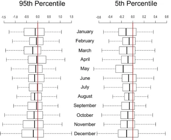
Figure 2 shows the results of the validation process: the monthly bias (i.e. difference between observed and estimated values) for the percentiles 5th_{and 95}th_{. We present only these values because}

(8)

they provide practitioners with a way to calculate 90% of the hourly variability of the wind resource. On average, this bias resulted -0.08 m/s for the 5th percentile and -0.11 m/s for the 95th_{percentile. By}

looking at the plot in Figure 2 we can clearly observe that the variation of the bias of the 5th percentile is relatively small, while it is more acute for the 95th_{, where the bias is above absolute 1 m/s. In essence,}

on average the bias of both percentiles is very low, and this indicates that we are able to provide planners with a reasonable estimate of the full range of variability of the wind speed (i.e. 90% of the time the wind speed is within this range).

Fig. 2: Monthly distribution of the bias of the estimated 5th and 95th percentiles.

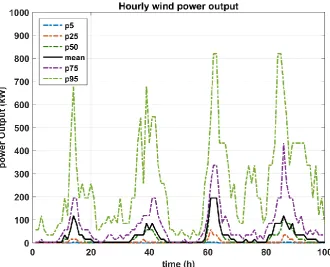
Figure 3 shows an excerpt of the generated time series with the mean wind speed (black line) and the percentile 25th_{, 50}th_{, 75}th_{and 90}th_{(dotted lines). In order to show the impact of the wind variability of the}

electricity generation, we calculated the energy output of a single Enercom turbine with a nominal power of 2.3 MW and 90 m hub height. The purpose of this test is only to show that considering the uncertainty around the mean wind speed is crucial for planners to identify correctly the interval of probability of the power output. For this reason, we considered a single turbine, which is often not a realistic scenario for wind farms, where multiple turbines are located relatively close to each other and factors such as the wake effect need to be considered to calculate the total power output. However, since we are only interested in showing the effect of considering uncertainty when computing the potential power output, considering a single turbine is sufficient. The results are shown in Figure 4.

In this plot we not only included the mean wind speed, but also all the percentiles we calculated in our study. Considering only the mean wind speed, certain time intervals seem productive. However, what we can tell by adding a measure of the local variability of the wind resource is that even in these intervals the productivity of the wind farm may be well below average, for certain years. This can be clearly identified using the confidence intervals we provide. This is a crucial information since it may allow planners to not only calculate the average power output, but also its upper and lower boundary and assign precise probability of occurrence to each of them. This certainly allows a very precise assessment of the risk involved in developing a site.

(9)

Fig. 3: Excerpt of the generated mean wind speed time-series (at 90 m AGL) and the corresponding percentiles.

Fig. 4: Excerpt of the generated mean power output time-series and the corresponding percentiles.

(10)

4. Conclusions

This research is an example of the use of statistical wind resource assessment for estimating hourly time-series, including a precise range of uncertainty. Estimating the wind resource at high spatio-temporal resolution using statistical methods is certainly much faster than with traditional methods based on computational fluid dynamics, as demonstrated in [4], and this makes this method useful for the industry. In fact, being able to provide practitioners with hourly confidence intervals at high spatial resolution can be advantageous not only for planning but also for wind farms operations.

The method presented here is based on machine learning and estimates the spatio-temporal pattern of the wind speed including a detailed uncertainty estimation, in the form of confidence intervals. With such a method practitioners are able to determine a priori the range of variability of the wind resource along the year, and in every mapped location. This may be useful to estimate the power production in specific weeks or months, but it cannot be used for forecasting. In fact, the results we generate are only accurate in providing a range of variation, not in providing the exact wind speed in future time intervals. Moreover, machine learning contrary to numerical weather prediction, is a data driven approach. This means that in areas with very low coverage of weather stations, for example in the Swiss Alps, its estimates are affected by a higher uncertainty. This could only be decreased by either adding weather observations or potentially using numerical wind flow models to increase the climatic information for these areas. The important thing to remember about statistical wind resource assessment, which makes it an effective method, is that it is able to estimate its own accuracy, thus allowing practitioners to spot problematic locations. This is very difficult to achieve with numerical weather prediction models.

5. Acknowledgment

The authors acknowledge the CTI - Commission for Technology and Innovation (CH), and the SCCER-FURIES - Swiss Competence Center for Energy Research - Future Swiss Electrical Infrastructure, for their financial and technical support to the research activity presented in this paper.

References

[1] P. Argyle and S. J. Watson, “Assessing the dependence of surface layer atmospheric stability on measurement height at offshore locations,” Journal of Wind Engineering and Industrial

Aerodynamics, vol. 131, pp. 88–99, 2014.

[2] M. Brower, Wind resource assessment: a practical guide to developing a wind project. John Wiley & Sons, 2012.

[3] G. T. Phillips, “Preliminary user’s guide for the NOABL objective analysis code. Special report, 15 June 1977-15 June 1978,” Science Applications, Inc., La Jolla, CA (USA), 1979.

[4] F. Veronesi, S. Grassi, and M. Raubal, “Statistical learning approach for wind resource assessment,” Renewable and Sustainable Energy Reviews, vol. 56, pp. 836–850, 2016. [5] H. Aksoy, Z. Fuat Toprak, A. Aytek, and N. Erdem Ünal, “Stochastic generation of hourly mean

wind speed data,” Renewable Energy, vol. 29, no. 14, pp. 2111–2131, Nov. 2004.

[6] W. Luo, M. C. Taylor, and S. R. Parker, “A comparison of spatial interpolation methods to estimate continuous wind speed surfaces using irregularly distributed data from England and Wales,” International Journal of Climatology, vol. 28, no. 7, pp. 947–959, 2008.

[7] L. Foresti, D. Tuia, M. Kanevski, and A. Pozdnoukhov, “Learning wind fields with multiple kernels,” Stochastic Environmental Research and Risk Assessment, vol. 25, no. 1, pp. 51–66, 2011. [8] M. Cellura, G. Cirrincione, A. Marvuglia, and A. Miraoui, “Wind speed spatial estimation for energy

planning in Sicily: A neural kriging application,” Renewable Energy, vol. 33, no. 6, pp. 1251–1266, 2008.

[9] Castellanos and V. I. Ramesar, “Characterization and estimation of wind energy resources using autoregressive modelling and probability density functions,” Wind Engineering, vol. 30, no. 1, pp. 1–14, 2006.

[10] K. Philippopoulos and D. Deligiorgi, “Statistical simulation of wind speed in Athens, Greece based on Weibull and ARMA models,” Int. J. Energy Environ, vol. 3, no. 4, pp. 151–158, 2009.

[11] A. Shamshad, M. A. Bawadi, W. W. Hussin, T. A. Majid, and S. A. M. Sanusi, “First and second order Markov chain models for synthetic generation of wind speed time series,” Energy, vol. 30, no. 5, pp. 693–708, 2005.

[12] P. Poggi, M. Muselli, G. Notton, C. Cristofari, and A. Louche, “Forecasting and simulating wind speed in Corsica by using an autoregressive model,” Energy conversion and management, vol. 44, no. 20, pp. 3177–3196, 2003.

(11)

[13] O. Ohashi and L. Torgo, “Wind speed forecasting using spatio-temporal indicators.,” in ECAI, 2012, pp. 975–980.

[14] F. Veronesi, S. Grassi, and M. Raubal, “Satellite data to improve the accuracy of statistical models for wind resource assessment,” presented at the EWEA 2015 Annual Event, Paris.

[15] B. Efron and R. J. Tibshirani, An introduction to the bootstrap. CRC press, 1994.

[16] National Oceanic and Atmospheric Administration (NOAA), “Global Surface Summary of the Day - GSOD.” 2016.

[17] P. W. Stackhouse, “Surface meteorology and solar energy,” 2011.

[18] J. Schulz, P. Albert, H.-D. Behr, D. Caprion, H. Deneke, S. Dewitte, B. Dürr, P. Fuchs, A. Gratzki, and P. Hechler, “Operational climate monitoring from space: the EUMETSAT Satellite Application Facility on Climate Monitoring (CM-SAF).,” Atmospheric Chemistry & Physics, vol. 9, no. 5, 2009. [19] J. J. Danielson and D. B. Gesch, “Global multi-resolution terrain elevation data 2010

(GMTED2010),” US Geological Survey, 2011.

[20] S. Grassi, S. Junghans, and M. Raubal, “Assessment of the wake effect on the energy production of onshore wind farms using GIS,” Applied Energy, vol. 136, pp. 827–837, 2014.

[21] H. Erich, Wind turbines: fundamentals, technologies, application, economics. New York: Springer, 2000.