Volume 17, Issue 1, January 2020
Computational Normative Decision Support
Structures of Forensic Interpretation in the
Legal Process
Alex Biedermann,* Silvia Bozza,** Franco Taroni,*** Joëlle Vuille****
© 2020 Alex Biedermann, Silvia Bozza, Franco Taroni, Joëlle Vuille Licensed under a Creative Commons
Attribution-NonCommercial-NoDerivatives 4.0 International (CC BY-NC-ND 4.0) license
DOI: 10.2966/scrip.170120.83
Abstract
networks). Such models, hereafter called normative decision support structures, can be operationally implemented through commercially and academically available software systems. These normative decision support structures represent core computational models that can be integrated as part of decision and litigation support systems, to help the participants of a legal process answer a variety of questions regarding complex strategic decisions.
Keywords
Decision theory, forensic science, dispute resolution, legal negotiation, Bayesian decision networks, normative decision policies, sequential decisions
* Faculty of Law, Criminal Justice and Public Administration, School of Criminal Justice, University of Lausanne, Lausanne, Switzerland, [email protected].
** Department of Economics, Ca’ Foscari University of Venice, Venice, Italy, [email protected]; Faculty of Law, Criminal Justice and Public Administration, School of Criminal Justice, University of Lausanne, Lausanne, Switzerland, [email protected].
*** Faculty of Law, Criminal Justice and Public Administration, School of Criminal Justice, University of Lausanne, Lausanne, Switzerland, [email protected].
1 Introduction
In light of the ever-increasing intricacy of legal practices, sound methodology to
support thinking and making decisions in practical cases is a topic of interest for
both researchers and practitioners. The central aspects of a given civil or criminal
case, in particular those over which disagreement exists, need to be thought
about in a structured way to enable insight and improve communication between
various participants in the legal process. This includes lawyer and client
relationships as well as the relationship between adversarial parties at trial.
Methodologies for analysing legal cases, and their implementation, are pivotal
topics for both practitioners and academics, because of the need to cope
coherently with the problem of decision-making under uncertainty. For example,
a party may need to decide whether to settle or plead guilty, whether to go to
trial or how to allocate resources (e.g., to the search of further information). Such
decisions place a party’s wealth, welfare or personal liberty at stake, and
attorneys must thus formulate legal tactics that appropriately reflect the party’s
preferences for or aversion to process outcomes. In litigation law, for example,
factors such as the costs of going to trial, and the uncertainties about possible
outcomes (verdicts) all need to be dealt with in a coherent whole. Such questions
involve all the ingredients of classic decision theory: feasible decisions, uncertain
states of nature, consequences (i.e., combinations of decisions and states of
nature) and a valuation of the desirability (or, worth) of consequences.1 Decision
theory is strongly rooted in economics2 and, following developments by several
leading business school groups in the middle of the last century, it has also
1 E.g., Howard Raiffa, Decision Analysis, Introductory Lectures on Choices under Uncertainty (Reading, Mass.: Addison-Wesley, 1968); Howard Raiffa and Robert Schlaifer, Applied Statistical Decision Theory (Cambridge, Mass.: MIT Press, 1961).
stimulated interest in the legal arena.3 This interest has steadily increased and has
been further strengthened, mainly since the 1980s, by the development of widely
available computer systems capable of processing the mathematical form of legal
decision models.4 Such systems are not intended to replace various
decision-makers in the legal process nor do such concepts claim to offer a comprehensive
descriptive account of the various aspects of the legal process that they seek to
model. Instead, such systems should best be considered as decision support
devices to assist in the analysis of selected aspects of the densely connected
network of factors upon which the outcomes of a case depend, at the level of
detail that the user considers appropriate. Thus, they offer a normative
perspective in the sense further discussed below.
The prototypical questions that have attracted wide interest among
decision-theoretic researchers and legal scholars relate to the conviction or
acquittal of defendants in the criminal trial, and the determination of the liability
of defendants in civil lawsuits. These are important but far end points of legal
processes. Decision theory, however, is a general theory for analysing how an
individual, facing the question of what decision to make in situations of
uncertainty, should proceed so as to insure coherence with that person’s
judgments and preferences among possible decision outcomes.5 In this paper, we
build on existing works on decision theory for strategic questions arising in the
legal context and then develop two extensions. The first is a translation of the
3 Alan Cullison, “Probability Analysis of Judicial Fact-Finding: A Preliminary Outline of the Subjective Approach” (1969) 1 University of Toledo Law Review pp. 538-698; John Kaplan, “Decision Theory and the Factfinding Process” (1968) 20(6) Stanford Law Review 1065-1092. 4 Stuart Nagel, Microcomputers as Decision Aids in Law Practice (New York: Quorum Books, 1987);
Stuart Nagel, Decision-Aiding Software and Legal Decision-Making: A Guide to Skills and Applications Throughout the Law (New York: Quorum Books, 1989).
5 Ronald Howard, “Decision Analysis and Law” in Marilyn Mac Crimmon and Peter Tillers
standard model of legal negotiations, commonly represented in terms of decision
trees,6 into Bayesian decision networks, also sometimes called influence
diagrams.7 Bayesian decision networks are a highly flexible modelling
environment that can be implemented using academically and commercially
available software systems. The second extension concerns results of forensic
examinations that may have an impact on trial outcomes, or intermediate steps
in the legal process. To operate this second extension, we will take advantage of
the fact that the use of graphical models, such as Bayesian networks and Bayesian
decision networks, is already a well-established area of research for analysing the
probative strength of forensic science results.8 Thus, the question of how to
logically connect reasoning models for legal negotiations and forensic results is
an area which offers much room for fundamental research.
By choosing decision-theoretic graphical models we emphasise that the
analyses pursued in this paper are normative,9 i.e. focusing on explicit reference
points against which one can compare one’s reasoning and conclusions in
practical situations that require a decision to be made.10 Stated otherwise, we will
not deal with the empirical question of whether people’s actual behaviour
conforms to the normative account of decision-making. There is, in fact,
substantial evidence that people’s intuitive and unaided reasoning generally
diverges from normative standards.11 While descriptive research is important to
6 E.g., Howard Raiffa, The Art and Science of Negotiation, How to Resolve Conflicts and Get the Best
out of Bargaining (Cambridge, Mass.: Belknap Press of Harvard University Press, 1982). 7 Uffe Kjærulff and Anders Madsen, Bayesian Networks and Influence Diagrams, A Guide to
Construction and Analysis (New York: Springer, 2008).
8 Franco Taroni et al., Bayesian Networks for Probabilistic Inference and Decision Analysis in Forensic
Science, 2nd ed., (Chichester: John Wiley & Sons, 2014).
9 Dennis Lindley, Making Decisions, 2nd ed. (Chichester: John Wiley & Sons, 1985).
10 Johnathan Baron, Thinking and Deciding (New York: Cambridge University Press, 2008, 4th ed.).
11 E.g., Terry Connolly, “Decision Theory, Reasonable Doubt, and the Utility of Erroneous
assess the extent to which people think and act coherently, we maintain that this
can only be achieved if the normative standpoints are first clarified (against
which observable behaviour can be compared), and this is what the normative
decision-theoretic structures developed throughout this paper seek to achieve.
We will call our models computational normative decision support structures
because our analyses, using formal approaches, focus on the conceptual
relationship between traditional interpretation of forensic science results and
strategic analysis in legal proceedings.
The paper is organized as follows. Section 2 briefly introduces the
graphical models for decision-theoretic analyses used in later parts of the paper,
i.e. decision trees and Bayesian decision networks (influence diagrams), using a
general example of plea bargaining from the defendant’s point of view. Readers
well acquainted with these concepts may skip this section. Section 3 starts with
an outline of how to state the general model of legal negotiations in terms of a
Bayesian decision network. Extensions regarding litigation costs, uncertainty
factors affecting these costs and other elements characterising the decision
problem are added gradually, with all decision-theoretic computations outlined.
It will be shown that Bayesian decision networks allow one to deal with formal
decision-theoretic calculations and incorporate notions such as perfect and
partial information. Section 3 will also outline the model structures to deal with
the results of forensic examinations and the connection of these models with the
standard models for decision analysis in the legal context, using the notions of
sequential decision analysis and normative decision policies. Discussion and
conclusions will be presented in Section 4.
2 Methods and notation
2.1 Decision trees
Decision trees are a general method to capture and convey the basic components
of a decision problem. For the purpose of illustration, imagine a defendant
(assisted by an attorney) who must decide between two actions. Denote them 𝑑1, accepting a plea of guilty on a reduced charge, and 𝑑2, letting the case go to trial.
Other decision cases will be studied in the main part of the paper (Section 3).
When making a decision, there may be uncertainty about the state of nature,
current or future. In the situation faced by the defendant, there may be
uncertainty about the trial outcome if he decides 𝑑2, i.e. going to court instead of
accepting a plea agreement (𝑑1). Let the two future legal conclusions (verdicts),
about which the defendant is uncertain at the time of deciding between 𝑑1 and
𝑑2, be denoted 𝜃1, for “guilty”, and 𝜃2, for “not guilty”. Note that here the focus
is on uncertainty about the legal conclusion that will be reached when applying
the law to the facts of the case. Such uncertainty cannot be eliminated, but it can
be measured by means of probabilities.12 We are not concerned here with the
various events that may have happened and that will form the basis for reaching
a conclusion at trial. This relates to another decision process by another
maker (e.g., the court), which is different from the viewpoint of the defendant
studied here.
Deciding 𝑑𝑖 in light of a state of nature 𝜃𝑗 leads to a consequence 𝐶𝑖𝑗. Thus,
in the hypothetical case considered here, 𝐶21 is the consequence of taking the case to trial (𝑑2) with the outcome that the accused is found guilty at the end of the
trial (𝜃1), whereas 𝐶22 is the consequence of taking the case to trial (𝑑2) with the outcome that the accused is found not guilty at the end of the trial (𝜃2). Note that
when taking 𝑑1, accepting the plea on a reduce charge, there is only a single
consequence, 𝐶1∙, that is the reduced charge as defined in advance. In particular,
since there will be no trial, there is no uncertainty about legal conclusions 𝜃1 and
𝜃2 that needs to be taken into account. The consequences 𝐶𝑖𝑗 in this example are
characterised in terms of years of imprisonment, denoted hereafter by PT(𝐶𝑖𝑗),
i.e. the prison time PT associated with consequence 𝐶𝑖𝑗. We acknowledge,
however, that this represents a simplified view, in the sense that there may be
further aspects that characterise a decision consequence. For example, if found
guilty, the defendant may lose his job, he may be disenfranchised etc. More
generally, to each consequence 𝐶𝑖𝑗 is associated a utility, denoted U(𝐶𝑖𝑗), or a loss,
denoted Lo(𝐶𝑖𝑗), quantifying or expressing the desirability or undesirability of
the incurred outcomes, respectively. In the case at hand, the loss is assumed to
be linear over the total range of years that can possibly result from a conviction.
Hence, it can be set numerically equal to the years of imprisonment, that is
Lo(𝐶𝑖𝑗) = PT(𝐶𝑖𝑗). Note, however, that losses can also be quantified differently.
For example, the undesirability of a conviction can be measured in monetary
terms. An example where the desirability of decision consequences is quantified
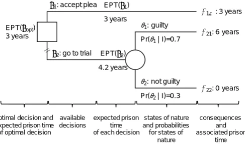
Figure 1: Decision tree for a defendant’s decision problem. The square represents the
available decisions 𝑑𝑖, i = {1, 2}. The circle represents the states of nature 𝜃𝑗 , j = {1, 2},
which determine the outcomes 𝐶2𝑗 if decision 𝑑2 is taken. Pr(𝜃𝑗|𝐼) represents the
probability of state of nature 𝜃𝑗 given information I. All consequences 𝐶 are valued in
terms of years of imprisonment. Decisions are compared on the basis of the expected
prison time, EPT. The decision branch which does not offer the smallest EPT, here 𝑑1,
is double crossed //.
In decision trees, the above decision-theoretic elements are captured as
shown in Figure 1. The actions available to the defendant, 𝑑1 and 𝑑2, are
described by the two branches that emanate from the trunk, shown as a square –
the decision node – on the far left-hand side. The circled node, also called chance
node, represents states of nature about which the decision-maker is uncertain.
There is a time order when going from left to right, because when deciding 𝑑2, two things can happen. Either, the fact-finder will find the defendant guilty, 𝜃1,
an event thought to occur with probability 0.7, or 𝜃2, the event of finding the
defendant not guilty, an event thought to occur with probability 0.3. At the far
right-hand side, the terminal states 𝐶 are shown, along with their associated evaluation of undesirability (in the case here losses in terms of years of
imprisonment). The chance node is labelled with the expected prison term, EPT,
of the decision 𝑑2 whereas the squared decision node is labelled with the
d1: accept plea
d2: go to trial
q1: guilty
q2: not guilty
C1・: 3 years
C21: 6 years
C22: 0 years Pr(q1 | I)=0.7
Pr(q2| I)=0.3 EPT(d2)
4.2 years EPT(d1) 3 years EPT(dopt)
3 years
optimal decision and expected prison time of optimal decision
available decisions
expected prison time of each decision
states of nature and probabilities for states of
nature
consequences and associated prison
expected prison term of the optimal decision 𝑑𝑜𝑝𝑡. In the analysis here, it is
considered that the optimal decision is the one which has the smallest EPT. For
the case studied here, the EPT associated with the decision to go to trial (𝑑2), is
4.2, and is obtained by summing over the possible states of nature the product of
the loss associated to each consequence 𝐶𝑖𝑗 (i.e., the prison time PT(𝐶𝑖𝑗)) and the
probability of the state of nature, that is:
EPT(𝑑2) = PT(𝐶𝑖𝑗) Pr(𝜃1|𝐼) + PT(𝐶22) Pr(𝜃2|𝐼) = 6 × 0.7 + 0 × 0.3 = 4.2.
The branch 𝑑1 has a smaller EPT, 3 years, which corresponds to the loss
associated to the consequence 𝐶1∙, the reduced charge. In summary, thus
EPT(𝑑1) < EPT(𝑑2) and it follows that the optimal decision is 𝑑𝑜𝑝𝑡 = 𝑑1.13 This is
in agreement with the assumption that the defence pursues the hypothetical
objective of minimizing the expected length of time the defendant will be
deprived of liberty. To some extent this helps illustrate why many defendants
accept guilty pleas even though they may assign only a moderate or low
13 The elicitation of probabilities for states of nature is often considered a tedious task, since decision-makers are asked to translate into numbers their personal beliefs, sometimes with an unrealistic level of precision. However, the decision-maker can perform a sensitivity analysis to provide a threshold for the required probability Pr(𝜃1|𝐼) with which the optimal decision
will change. In the current example, one may easily observe that the limiting value for Pr(𝜃1|𝐼)
is equal to 0.5: as long as the event that the court will find the defendant guilty is considered to be more probable than the event that the court will render a verdict of not guilty, the optimal decision is 𝑑1. The assignment of losses is another intricate task. Clearly, one may observe that
probability of being convicted if the case went to trial: because the sentence in
case of a conviction may be very severe (or perceived as such), even a low
probability for a conviction will be sufficient to ‘outweigh’ the sentence
associated with the guilty plea. While this is a purely formal view, we concede
that in practice defendants may prefer a guilty plea for other reasons, too.
Let us emphasise again that evaluating the undesirability of decision
consequences directly in terms of prison time was a choice made for the sole
purpose of providing an example, and that other loss functions associating a
higher severity to adverse outcomes can be built. This may lead to losses
expressing nearly infinitely undesirable consequences that would make going to
trial unadvisable even in presence of a very low probability of an unfavourable
verdict.14 Moreover, going to trial may be perceived as a highly aleatory
undertaking, with sentence length and probabilities for verdicts being difficult to
assess, thus making the guilty plea with its sure consequence the preferable
option. Specifically, if the defendant refuses to quantify uncertainty (about states
of nature; here verdicts), or refuses to run the risk of incurring the worst
consequence associated with going to trial (especially if 𝐶21 represents a severe sentence), and hence accept the guilty plea (𝑑1), such a strategy would amount to
minimising the maximum loss. This is a non-probabilistic decision criterion also
known in literature as minimax.15 It is important to note that such an alternative
consideration is not in conflict with the general decision theoretic approach
14 The reason for using the term “nearly infinitely undesirable consequences” is that the axiomatic foundation for the existence of a utility function we refer to requires that there do not exist infinitely undesirable consequences. Otherwise, no matter how small the probability of a conviction is, one will always prefer to avoid going to trial.
considered here: the basic decomposition of the decision problem outlined at the
beginning of this section, summarised graphically in Figure 1, remains the same.
The point of view of the prosecution may be different in that they may
seek to maximise the expected prison time, and hence the expected length of time
the offender is kept away from society. But again, we emphasise that there may
be other – concurrent – objectives in prosecution decision-making, beyond the
scope of the generic introductory example chosen here. Our current
demonstration only focuses on a single objective and how this single objective is
conceptualised. The reader may use other values for probabilities and losses (e.g.,
different sentence lengths) as required, but should be aware of the fact that this
may impact on the EPT of the two decisions, and hence 𝑑𝑜𝑝𝑡. For example, for
any plea of guilty on a reduced charge greater than 4.2 years, while keeping the
other assignments as defined above, the optimal decision is 𝑑𝑜𝑝𝑡 = 𝑑2.
2.2 Bayesian decision networks (influence diagrams)
While decision trees (Section 2.1) provide a static summary of the main features
of a decision analysis, such as probabilities and (expected) utilities, Bayesian
decision networks (BDNs) provide a more flexible and dynamic, but also more
compact modelling framework. BDNs extend Bayesian networks by including
rectangle nodes for representing decision variables and diamonds for
representing utility functions.16 To illustrate the main components of BDNs,
consider again the defendant’s decision problem introduced in Section 2.1.
Figure 2 represents the main aspects of this case in terms of a BDN. Rather than
presenting a full and simultaneous display of all “routes” that may follow from
a decision (as shown in Figure 1), variables in a BDN are represented by single
nodes. For example, instead of having a branch for each decision 𝑑𝑖 in a decision tree, a BDN concentrates all decisions in a single node (here node D). The
expanded node D in Figure 2(ii) summarises the EPT associated with each
decision 𝑑𝑖. These EPT values correspond to the values attached to the branches
𝑑𝑖 of the decision tree (Figure 1). Note that the BDN in Figure 2 is the simplest
possible model structure as it involves exactly one node for each node category,
i.e. nodes for states of nature (also called chance nodes), decisions and utilities.
More elaborate models will be introduced in later sections. Note that the links
pointing from nodes D and 𝜃 to PT mean that the “goodness” of a decision, here
decision 𝑑2, is dependent on the future state of nature 𝜃 (i.e., the trial outcome). In particular, the node PT contains a table that specifies a prison term (in years)
for each combination of a decision 𝑑𝑖 and a trial outcome 𝜃𝑗, for i,j = {1,2}.
Bayesian decision networks are fairly flexible, as is illustrated by Figure 2
(iii), which shows an alternative network structure. In this model, the states of
nature 𝜃𝑗 depend on the decisions 𝑑𝑖. In particular, there is an additional state of
nature 𝜃3, ‘no trial’, that is the situation in which 𝑑1 (accept plea agreement) is chosen. The structural relationship 𝐷 → 𝜃 thus allows us to specify probabilities
that depend on propositions, Pr(𝜃𝑗|𝑑𝑖). So, for the case in which the defendant
accepts the plea (𝑑1), the conditional probabilities for the states of nature θj are
Pr(𝜃𝑗|𝑑1) = {0,0,1}, where 𝜃1=guilty, 𝜃2=not guilty and 𝜃3=no trial. And, clearly,
if the decision is to prosecute (𝑑2), the probabilities are Pr(𝜃𝑗|𝑑2) = {0.7,0.3,0}, for
j = {1, 2, 3}. The utility node17PT contains the values (prison terms) 6 if 𝜃
1 (guilty)
holds, 0 if 𝜃2 (not guilty) holds and 3 if 𝜃3 (no trial) holds. Note that the latter
assignment, PT(𝐶1∙) = 3, corresponds to the reduced charge associated with the accepted plea.
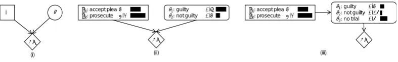
Figure 2: Bayesian decision networks for the defendant’s decision problem introduced
in Section 2.1. The node 𝜃 represents the uncertain states of nature (i.e., trial outcomes),
the diamond shaped node PT the evaluation of the consequences (quantified in terms
of prison term), and the squared node D the available actions. Figure (i) shows the
general network structure whereas Figure (ii) shows the nodes D and 𝜃 in full detail
for a situation in which the defendant expects a guilty verdict at the end of the process
to occur with probability 0.7 and a not guilty verdict with probability 0.3. Node D
shows the expected prison term (EPT) for the two decisions 𝑑2 and 𝑑2. Figure (iii)
shows an alternative network structure leading to the same EPT, the sole difference
being the introduction of an additional state of nature 𝜃3 to account for the situation
of no trial being held when decision 𝑑1 is taken.
3 Normative decision structures
3.1 Standard model of legal negotiations
Consider now a standard model of legal negotiations through the case of a
hypothetical damage suit in the amount of €150,000. The plaintiff faces the decision of whether to accept an out-of-court settlement (decision 𝑑1), or to bring
the lawsuit to trial (decision 𝑑2). The plaintiff can either win the case (𝜃1), or lose
the case (𝜃2). Suppose that the plaintiff’s current assessment of his probability of
D q
PT
d1: accept plea3
d2: prosecute 4.2
PT
q1: guilty 0.7 q2: not guilty 0.3
(i) (ii)
d1: accept plea3
d2: prosecute 4.2
PT q1: guilty 0.3 q2: not guilty 0.15 q3: no trial 0.5
winning the case is 0.8.18 Using notation introduced above, we can write this as
Pr(𝜃1|𝐼) = 0.8, where I denotes the plaintiff’s current state of information. By
coherence, the probability of losing the case is Pr(𝜃2|𝐼) = 0.2, again considered from the plaintiff’s point of view. Note that in this case the probabilities of states
of nature are not conditioned on decisions. For the time being, we will leave aside
considerations of litigation costs; we will introduce these step by step later on.
The purpose at this point is to draw the attention solely to the notion of the
expected value of going to trial, to embody the essence of the problem. In the case
here, we suppose that the consequence of a decision is entirely described in
monetary terms (monetary value, MV), and that the utility function is linear so
that the utility can be set to be numerically equal to the monetary value, that is
U(MV(𝑑𝑖, 𝜃𝑗)) = MV(𝑑𝑖, 𝜃𝑗). Moreover, we suppose that the decision-maker is
willing to act on the basis of expected monetary value (EMV), or at least is
interested in this value prior to making a decision based on considerations going
beyond those explicitly taken into account at this juncture. As in the previous
sections, we emphasise that action based on EMV is an assumption subject to
discussion, though it does not impact on the principle of the proposed analyses.
It is perfectly feasible, for example, to choose another utility function to account
for individual preferences according to which changes in the utility of very low
or very high monetary values are notlinear.
In the above framework, the optimal decision 𝑑𝑜𝑝𝑡 will be the one at which
the EMV attains its maximum, that is
EMV(𝑑𝑜𝑝𝑡) = max
𝑖 EMV(𝑑𝑖).
We can write the EMV associated with going to trial, for the plaintiff, as
follows:
EMV(𝑑2) = MV(𝑑2, 𝜃1) × Pr(𝜃1|𝐼) + MV(𝑑2, 𝜃2) × Pr(𝜃2|𝐼) (1)
= (€ 150,000) × 0.8 + (€ 0) × 0.2 = € 120,000.
Note that when deciding 𝑑1, there will be no trial, and the plaintiff accepts
the out-of-court settlement as given by the monetary value x. It is not necessary
at this point, to be explicit about x. It suffices to note that EMV(𝑑1) = 𝑥 and the plaintiff will decide 𝑑1 whenever EMV(𝑑1) > EMV(𝑑2), that is the settlement offer
𝑥 > € 120,000. In other words, the plaintiff will decide to go to trial if the
expected monetary output, that is the target amount of € 150,000, discounted by
probability, is greater than the sure return x from the out-of-court settlement.
3.2 Influence diagrams for the standard model of legal negotiations
In a more realistic perspective, the MV introduced in Section 3.1 should account
for the cost of litigation 𝑙 = L(𝑑𝑖, 𝜃𝑗), taken here as the cost incurred by legal
representation. Other specific costs may be included in the analysis without loss
of generality. Under the reasonable assumption of additivity, since costs are
quantified in monetary terms, the monetary value MV can be taken as the net
amount which the decision-maker will receive, one has
The expected monetary value of decision 𝑑1 will become
EMV(𝑑2) = MV(𝑑2, 𝜃1, 𝑙) × Pr (𝜃1|𝐼) + MV(𝑑2, 𝜃2, 𝑙) × Pr (𝜃2|𝐼)
= ∑[MV(𝑑2, 𝜃𝑗) − L(𝑑2, 𝜃𝑗)]
2
𝑗=1
× Pr(𝜃𝑗|𝐼). (3)
In some circumstances, the cost of litigation can be assumed to be
independent on the outcome of the trial, that is L(𝑑2, 𝜃1) = L(𝑑2, 𝜃2) = L(𝑑2).
Under this assumption, expression (2) can be simplified as
MV(𝑑𝑖, 𝜃𝑗, 𝑙) = MV(𝑑𝑖, 𝜃𝑗) − L(𝑑𝑖). (4)
Litigation costs will then combine naturally with the EMV by
subtraction,19 that is:
EMV(𝑑2) = [MV(𝑑2, 𝜃1) − L(𝑑2)] × Pr (𝜃1|𝐼) + [MV(𝑑2, 𝜃2) − L(𝑑2)] × Pr (𝜃2|𝐼)
= ∑ MV(𝑑2, 𝜃𝑗) 2
𝑗=1
× Pr(𝜃𝑗|𝐼) − L(𝑑2). (5)
In the remainder of this paper, it will be assumed that litigation costs are
independent of the outcome of the trial. It is possible, however, to avoid this
19 It is important to note that this is valid only under the assumption of linearity of the utility function. In fact, one has U(MV(𝑑𝑖, 𝜃𝑗, 𝑙)) = MV(𝑑𝑖, 𝜃𝑗, 𝑙) = MV(𝑑𝑖, 𝜃𝑗) − L(𝑑𝑖). If, however, the
utility function is not linear, U(MV(𝑑𝑖, 𝜃𝑗, 𝑙)) ≠ MV(𝑑𝑖, 𝜃𝑗, 𝑙) = MV(𝑑𝑖, 𝜃𝑗) and the assumption of
assumption and adapt the proposed BDNs accordingly as explained later in this
section.
One way to translate the current analysis into an influence diagram
consists in reusing the structure of the BDN shown in Figure 2(i) and to change
the definition of the nodes D and 𝜃 according to the elements of interest here, i.e. decisions 𝑑1 (out-of-court settlement) and 𝑑2 (pursue litigation), and states of
nature 𝜃1 (win trial) and 𝜃2 (lose trial). Note also that the definition of the utility
node, denoted G here, shorthand for “gain” understood in a broad sense as
defined below, has changed. The resulting model is shown in Figure 3(i). Note
that the node G contains the utility function expressed as before in terms of net
monetary values: MV(𝑑2, 𝜃1, 𝑙) = € 150,000 − € 20,000 = € 130,000, that is the
“gain” of winning the trial minus the litigation cost, MV(𝑑2, 𝜃2, 𝑙) = − € 20,000,
i.e. no “gain” when losing the case and incurring the litigation cost, and MV(𝑑1) = € 𝑥, i.e. the offered out-of-court settlement. For the purpose of the current
discussion, let x be € 90,000. Note also that when 𝑑1 is selected, there is no consideration of the variable 𝜃, the outcome of trial. The EMV of going to trial for
the plaintiff’s perspective thus is:
EMV(𝑑2) = (€ 150,000) × 0.8 + (€ 0) × 0.2 − € 20,000 = € 100,000. (6)
So, EMV(𝑑2) > EMV(𝑑1) and the plaintiff would refuse the out-of-court settlement in the amount of € 90,000. Note that we do not deal here with the
psychological dimension of the decision, in particular the fact that people may be
inclined to prefer an out-of-court settlement of € 90,000 that is certain (decision
𝑑1) rather than opt for 𝑑2 which involves a probability of 0.2 to incur the litigation
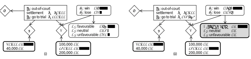
Figure 3: Bayesian decision networks for a standard model of legal negotiations. The
squared decision node D has states 𝑑1 (accept out-of-court settlement) and 𝑑2 (pursue
litigation at trial). The chance node 𝜃 has two states 𝜃1 (win trial) and 𝜃2 (lose trial). In
Figure (i), the node G quantifies all monetary aspects (e.g., costs, settlements, etc.) of
the consequences of decisions. In Figure (ii) and its expanded representation (iii),
distinct nodes L, S and G are used to specify, respectively, litigation costs, out-of-court
settlement amount and court-ordered settlement (verdict) in the event of winning trial.
Node D in Figure (iii) shows the EMV of each decision whereas node 𝜃 shows the
plaintiff’s probabilities for the various trial outcomes.
Although being a compact model, Figure 3(i) may be impractical because
the monetary values specified in the node G fuse different aspects of the problem,
such as litigation costs and gain in case of succeeding at trial. To enhance clarity
and exert better control over the different features, it is possible to introduce
distinct utility nodes for each monetary factor. This is shown in the BDN in Figure
3(ii) where the node D has child nodes L for the cost of litigation, and S for the
out-of-court settlement offer. In this model, the table of the node L specifies
− € 20,000 in the event of deciding 𝑑2 (pursuing the damage suit at trial). A
value of € 0 is specified in the event of 𝑑1, not going to trial, because it is assumed that this decision will incur no further litigation costs. A value different from 0
may be chosen, however, to account for costs of option 𝑑1 other than legal fees,
if required. Specifying the BDN in this way using, for example, a Bayesian
D q
G L
S
D q
G
(i) (ii)
d1: out-of-court
settlement € 90,000 d2: go to trial€100,000
q1: win 0.8
q2: lose 0.2
G L
S
network software such as HUGIN,20 leads to model output shown in expanded
version in Figure 3(iii).21 The decision node displays the EMV of the options 𝑑
1
and 𝑑2, and the chance node 𝜃 shows the plaintiff’s probabilities for the trial outcomes 𝜃1 and 𝜃2. It may be argued that none of these results are original,
because they may also be obtained using paper and pencil. It is relevant,
however, to pursue the development of these models stepwise, starting with
simple formats, in order to lay bare their constructional logic and demonstrate
that their output can be trusted. This represents an important preliminary step to
more advanced network structures for which the underlying calculations,
without computational support, become increasingly complex. The next section
illustrates the ease with which further features can be added.
3.3 Uncertainty about verdicts and litigation costs
A restriction of the models introduced so far is that factors such as the amount in
case of winning at trial (e.g., node G, Figure 3) and litigation costs are considered
fixed or known monetary values. However, at the time of making a decision, the
plaintiff may be uncertain about the length of the process and the court-ordered
settlement (i.e., the amount granted in case of a verdict favourable to the
plaintiff). We now point out how BDNs can readily handle such additional
sources of uncertainty.
Start by considering uncertainty about the litigation costs. These may
crucially depend, for example, on process length and case complexity. For the
purpose of illustration, suppose that the plaintiff considers that – given
consideration of the case as a whole – it is more probable than not that litigation
costs will be twice as high, that is € 40,000, rather than € 20,000 as in the previous
20 https://www.hugin.com; Kjærulff and Madsen, supra n. 7.
section. How does this affect the EMV of the decision 𝑑2 of going to trial? Let us assume that the plaintiff wishes to consider two different cases, i.e. litigation costs
of € 20,000 with probability 0.4, and € 40,000 with probability 0.6. The reader may consider other amounts and associated probabilities. The expected cost of
litigation thus is: (€ 20,000) × 0.4 + (€ 40,000) × 0.6 = € 32,000. Using this result in Equation (5), the EMV of going to trial for the plaintiff’s perspective thus
becomes:
EMV(𝑑2) = (€ 150,000) × 0.8 + (€ 0) × 0.2 − (€ 32,000) = € 88,000. (7)
Since the expected cost has increased by € 12,000, the EMV of decision 𝑑2
has decreased by the same amount. In particular, note that now EMV(𝑑2) < EMV(𝑑1) so that the out-of-court settlement € 90,000 becomes more
advantageous – it becomes the optimal decision – for the plaintiff, although the
plaintiff may consider this difference to be rather small. The proposed BDN can
be further developed to acknowledge for more realistic settlements where the
cost of litigation is a function of the process length. For example, one may
consider the litigation cost to be proportional to the fee per hour of a lawyer, by
adding a node to acknowledge for the expected length of the trial.
Next, consider uncertainty about the amount granted in case of a verdict
favourable to the plaintiff. Assume, for example, that the party considers three
possible amounts granted or court verdicts, € 100,000, € 150,000 and € 200,000,
with associated probabilities 0.3, 0.6 and 0.1. Thus, the fixed MV(𝑑2, 𝜃1) in
Equation (5) must be replaced by the expected monetary value, that is the sum of
the three outcomes weighted by their probability, that is (€ 100,000) × 0.3 + (€ 150,000) × 0.6 + (€ 200,000) × 0.1 = € 140,000. Inserting this result in
EMV(𝑑2) = (€ 140,000) × 0.8 + (€ 0) × 0.2 − (€ 32,000) = € 80,000. (8)
Thus, uncertainty about the amount of the court-ordered settlement has
led to a further decrease of the EMV, in addition to that incurred by uncertainty
about legal fees, so that there is now a more clear-cut difference with respect to
the EMV of 𝑑1, which is given by the out-of-court settlement amount of € 90,000.
To track the above results in a BDN, consider an extension of the model in
Figure 3(ii), shown here in Figure 4. This network contains an additional node L′
with two states 40,000 and 60,000 to which unconditional probabilities 0.4 and
0.6 are assigned. This node models the different litigation costs and the plaintiff’s
probabilities for these costs in case decision 𝑑2 is made. Adding node L′ as a
parent for L requires a modification of the node table of L so that it will copy the
negative value22 of the current state of L′ when the condition 𝐷 = 𝑑
2 holds, and
the value 0 otherwise. Software environments such as Hugin offer a rich syntax
(e.g., if-then expressions) to define functions in this way. Similarly, there is an
additional node G′, acting as a parent node for G. The states of G′ correspond to
the different court-ordered settlements, whereas the associated node probability
table contains the plaintiff’s probabilities for those outcomes in the event decision
𝑑2 is made. The node table of G is defined23 such that it copies the current value
of G′ in the case where both 𝐷 = 𝑑2 and 𝜃1 holds, and the value 0 otherwise.
22 A negative value is specified here because in Hugin utility nodes are considered as additive contributions to the utility function.
Figure 4: Extended BDNs for a standard model of legal negotiations. The nodes D, 𝜃,
S, L and G are defined as in Figure 3. Nodes L′ and G′ are extensions to deal with
uncertainty about, respectively, litigation costs and the trial verdict.
Figure 4(ii) shows a schematic illustration of the compiled network. The
node G′ is fixed (i.e., instantiated) to the state € 150,000, highlighted with a bold border line. This corresponds to a situation in which there is no uncertainty about
the court-ordered verdict. In turn, the node L′ is left uninstantiated so as to allow
for uncertainty about the litigation costs. For such a situation, the node D shows
that the EMV of decision 𝑑2 is € 88,000, which corresponds to the value found
through Equation (7). The network shown in Figure 4(iii) shows a situation that
allows for uncertainty about the court-ordered settlement, which is achieved by
leaving the node G′ uninstantiated. The EMV of decision 𝑑2 then is € 80,000, which corresponds to the result given by Equation (8).
3.4 The notion of perfect information (PI)
The previous sections have illustrated that the major factor rendering
decision-making hard is uncertainty about the state of nature 𝜃, for if we knew whether
𝜃1 (win) or 𝜃2 (lose) holds, choosing between 𝑑1 and 𝑑2 is more straightforward.
In the special case where other factors (e.g., litigation costs) could be considered
fixed (i.e., without uncertainty), it would even be possible to tell which decision
would offer the most desirable outcome within the stated modelling
assumptions. Therefore, any information capable of reducing uncertainties about
the states of nature, that is directing associated probabilities towards 0 and 1, is
of particular interest to decision-makers. One notion that is often encountered in
D q G L S (i) G’ L’
d1: out-of-court settlement € 90,000 d2: go to trial€ 80,000
q1: win 0.8
q2: lose0.2
G L
S
(iii) 20,000 0.4
40,000 0.6
100,0000.3
150,0000.6
200,0000.1 d1: out-of-court
settlement € 90,000 d2: go to trial€ 88,000
q1: win 0.8
q2: lose0.2
G L S (ii) 100,0000.0 150,000 1.0 200,0000.0
20,000 0.4
this context is perfect information (PI). This represents an element that is
completely informative about the propositions of interest (i.e., information that
would allow one to know which proposition is true). A crucial question is,
however, how valuable such data or information is. This question is pursued
below. Although it may be considered a hypothetical question, it is useful as a
starting point for thinking about the more general issue of data that are only
partially informative (i.e., imperfect). Such data do not allow us to establish with
complete certainty which state of nature actually holds, a property that typically
applies to forensic science results.
Perfect information can lead to two different outcomes. In one case, perfect
information would establish 𝜃1, i.e. winning the case. The best decision then is
𝑑2, pursuing the dispute, because the outcome will be a verdict of € 150,000,
from which the litigation costs of € 20,000 must be subtracted. The second possibility is that perfect information establishes 𝜃2, in which case decision 𝑑2
would incur the litigation costs of € 20,000, and no “gain”, whereas 𝑑1 would lead to the out-of-court settlement of € 90,000 (a situation in which no litigation
cost is assumed). But again, the states of nature are unknown, so at best one can
consider one’s expected outcome (monetary value) with perfect information
(EMVPI), defined as follows:
EMVPI = ∑[max
𝑖 (MV(𝑑𝑖, 𝜃𝑗) − L(𝑑𝑖))] 2
𝑗=1
× Pr(𝜃𝑗|𝐼). (9)
In the example considered here, this results in (€ 90,000 − € 20,000) × 0.8 + (€ 90,000) × 0.2 = € 122,000. Stated otherwise, the expected outcome with
perfect information is obtained by summing over the possible states of nature (or
associated with the optimal decision – weighted by the probability of the state of
nature.24
The EMVPI can be compared to the EMV of the optimal decision without
perfect information. For a case in which the verdict is taken to be constant at
€ 150,000, and the litigation cost fixed to € 20,000, the decision 𝑑2 was found to
be optimal, with an EMV of € 100,000, found through Equation (6) and also
shown in Figure 3(iii). The result of this comparison is the expected value of perfect
information (EVPI), that is € 22,000. It is often referred to as the maximum price
that one should be willing to pay for obtaining such perfect information. More
formally, it is defined as follows:
EVPI = EMVPI−EMV(𝑑𝑜𝑝𝑡). (10)
where dopt is the optimal decision without additional information, also
sometimes called the a priori optimal action.
The EVPI does not correspond to a particular state of a BDN, and hence
cannot directly be read off the graph.25 Rather, Equation (10) shows that the EVPI
is the result of a comparison of different situations, and those can be displayed
separately. As is illustrated by Figure 5, for example, one can determine the
optimal decisions and their associated EMVs under assumptions of perfect
information, which is needed to calculate the EMVPI, as part of the EVPI. The
added value of BDNs thus is to provide a unified environment in which one can
break down abstract formulae, such as Equation (9), into their constituting
24 Note that the procedure is general and also holds for n hypotheses.
components, which may otherwise be more difficult to achieve, and more prone
to error.
Figure 5: Extended BDNs for a standard model of legal negotiations. The nodes D, 𝜃,
S, L and G are defined as in Figure 3. Nodes L′ and G′ are extensions to deal with
uncertainty about, respectively, litigation costs and the verdict, fixed here to € 20,000
and € 150,000, respectively. Figure (i) shows a situation in which it is supposed that
perfect information about the state of nature is available, in particular that 𝜃1 holds
(node shown with grey shading). The optimal decision in this case is 𝑑2, leading to a
MV of € 130,000. In Figure (ii), the state 𝜃2 is supposed to hold. In this case the optimal
decision is 𝑑1 with outcome € 90,000. All instantiated nodes are highlighted with a
bold border line.
3.5 Expected value of partial information (pI)
In legal practice, it is often the case that a party has the option of seeking further
evidence that may have a bearing on the assessment of probabilities for trial
outcomes. Typically, information that may be gathered in real cases is not such
as to establish clear-cut values of 0 and 1 for the probabilities of the states of
nature as is supposed by perfect information (Section 3.4). Let us denote such
evidence partial information (pI).26 To assess the expected value of less than perfect
information, one needs to consider the effect that partial information has on one’s
probabilities for the relevant states of nature 𝜃. Given the probabilistic graphical
26 Here, the lower-case letter “p” denotes “partial” as compared to the capital letter “P” used to denote “perfect” in Section 3.4.
d1: out-of-court
settlement € 90,000
d2: go to trial€-20,000
q1: win 0.0 q2: lose 1.0
G L
S
20,000 1.0
40,000 0.0
100,0000.0 150,000 1.0
200,0000.0
d1: out-of-court
settlement € 90,000
d2: go to trial€130,000
q1: win 1.0 q2: lose 0.0
G L S 100,0000.0 150,000 1.0 200,0000.0 20,000 1.0
modelling framework used in this paper, this operation is naturally operated
through Bayes’ theorem.27 The procedure is outlined below. A forensic example
is given in Section 3.6.
Consider first that the optimal decision 𝑑 with partial information E, say
𝑑𝑜𝑝𝑡|𝐸, is the one that maximises the EMV calculated on the basis of the posterior
probabilities for the trial outcomes 𝜃 once the partial information E is available,
say Pr(𝜃|𝐸). Formally, thus, 𝑑𝑜𝑝𝑡|𝐸 is the decision at which the EMV attains its
maximum:
EMV(𝑑𝑜𝑝𝑡|𝐸) = max
𝑖 EMV(𝑑𝑖|𝐸) (11)
= max
𝑖 ∑[MV(𝑑𝑖, 𝜃𝑗) − L(𝑑𝑖)] × Pr(𝜃𝑗|𝐸) 2
𝑗=1
.
For shortness of notation only, we leave aside relevant information I from
notation and assume that there are fixed monetary values for the trial verdict in
case of winning, that is MV(𝑑2, 𝜃1), and the litigation costs L(𝑑2). Also, the
out-of-court settlement has a fixed value MV(𝑑1), which is independent of 𝜃, with no
associated litigation cost.
Equation (11) provides the guide to action in case the decision-maker
knows what kind of information E has been obtained, and hence posterior
probabilities Pr(𝜃𝑗|𝐸) are available. However, information E may take various
different forms (i.e., 𝐸𝑘, for k=1,2,...,n), so that prior to obtaining E the
decision-maker should take into account these possible outcomes 𝐸𝑘, along with an
expression of the associated uncertainty, in terms of probabilities. This leads to
the expected monetary value with partial information(EMVpI):
EMVpI = ∑ max
𝑖 EMV(𝑑𝑖|𝐸) × Pr(𝐸) (12) 𝐸
Equation (12) involves the multiplication of results in (11) by Pr(𝐸) over
the various possible forms that the information E can take.28 The difference
between this result and the EMV without information E is the expected value of
partial information(EVpI):
EVpI = EMVpI − max
𝑖 EMV(𝑑𝑖), (13)
where max
𝑖 EMV(𝑑𝑖) is EMV(𝑑𝑜𝑝𝑡), prior to the partial information E.
3.6 Example: EMV of partial forensic information
To illustrate the consideration of partial information with a forensic connotation,
suppose that E refers to the report of a forensic document examiner. Forensic
document examinations focus on a variety of aspects, such as physical document
examinations or comparative handwriting examinations. The results of such
examinations may help inform about document authenticity, for example, which
may be a key issue in a litigation case. Assume that the conclusion of the report
of the forensic scientists takes one of the following three different forms: findings
(i.e., evidence) favourable to the plaintiff (𝐸1), neutral findings (i.e., favouring
28 Note that the sum in Equation (12) may be replaced by an integral to deal with continuous
neither party; 𝐸2), and findings favourable to the defendant (𝐸3). Note that this is a general way of looking at the forensic scientist’s work, comparable to that of
other specialists and consultants that may be contacted as part of the legal
process.
What exactly forensic and other specialists are consulted for is a crucial
point that is worthy to be defined in more detail. In particular, we emphasize that
the issue here is not the use of results of forensic examinations to help inform
about intermediate propositions such as “the questioned document was signed
by the defendant” versus “an unknown person signed the questioned
document”, or “the questioned document was printed with the defendant’s
device” versus “an unknown printer was used”. Such propositions are used in
conventional evaluations of forensic results.29 Here a different uncertain
proposition is of interest: it is the outcome of the lawsuit, denoted 𝜃, which is the uncertain event bearing on the decision analysis.30
The decision analyst thus is directed to think about how the forensic report
E informs the party about θ, the verdict at the end of the trial. Let us emphasise
again that the question here is not one of weight of evidence for results of forensic
examinations, a notion concerned with propositions representing competing
versions of an event of interest. The focus here is the impact on verdicts, i.e. how
a given forensic conclusion will impact, as judged by the litigant, the relative
probabilities of the two possible ultimate trial outcomes. In a formal framework,
29 Colin Aitken and Franco Taroni, Statistics and the Evaluation of Evidence for Forensic Scientists, 2nd ed. (Chichester: John Wiley & Sons, 2004); Franco Taroni et al., Data Analysis in Forensic
Science: a Bayesian Decision Perspective (Chichester: John Wiley & Sons, 2010); see also supra n. 12.
a logical way to track this question is through Bayes’ theorem. With the prior
probabilities Pr(𝜃), obtaining the posterior probabilities Pr(𝜃|𝐸) requires the
consideration of the probabilities for E given 𝜃, Pr(𝐸|𝜃). Suppose the following values: Pr(𝐸𝑖|𝜃1) = {0.9,0.05,0.05} and Pr(𝐸𝑖|𝜃2) = {0.1,0.05,0.85}, for i = 1, 2, 3.
These assignments express the view that a forensic finding favourable to the
plaintiff (𝐸1) is more probable if the case in fact turns out favourably for the plain-
tiff (𝜃1), rather than unfavourably (𝜃2). The assignment also conveys the view that
a result unfavourable for the plaintiff (𝐸3) is more probable if the case in fact turns out unfavourably for the plaintiff (𝜃2), rather than favourably. It is also
considered that a “neutral” forensic result (𝐸2) is obtained with the same probability under each state of nature 𝜃. Note that these probabilities are also
sometimes interpreted as a consideration of an expert’s reliability. This is
comparable to other contexts where, for example, expert evidence is used to
inform about states of nature such as the presence or absence of oil or gas on a
potential mining site, or the commercial success of a new product introduced on
the market.
Clearly, finding the EVpI through Equation (13) with the above
assignments is a tedious task. However, we can illustrate the support provided
by computationally implemented Bayesian decision networks. They can either
break down the computation into smaller chunks or even provide the result in a
single step. The latter may be preferable if efficiency is required, whereas the
former may be of interest if intermediate results (e.g., the optimal decision and
associated EMV for a given result E) need to be inspected. This may be valuable
when consulting with a client because it will allow the analyst to work through
the decision network together with the client to demonstrate how the optimal
decision may change in different circumstances, and that the analyst has
seriously assessed each aspect of the client’s case. Below, we briefly outline both
Start by considering the computation of parts of the EVpI using the BDN
shown in Figure 6(i). It contains an additional chance node for the possible
forensic findings E, specified as a child node of 𝜃 (trial outcome). The conditional probabilities Pr(𝐸|𝜃) are as assigned above. Figure 6(i) shows the BDN in its
initial state, with nodes G′ and L′ fixed to, respectively, € 20K and € 150K. The node E shows the marginal probabilities for the various forms that the forensic
report may take. These values are one element needed for the EMVpI (Equation
(12). Further elements are posterior probabilities for 𝜃 and the EMV of the optimal decision given a particular posterior probability distribution over 𝜃.31
This is illustrated in Figure 6(ii) for the situation in which the outcome 𝐸1, a favourable forensic report (for the plaintiff’s position), is obtained: it is shown
that the posterior probability Pr(𝜃1|𝐸1) increases to 0.973 and the optimal
decision is 𝑑2, with an EMV of € 125,946. One can proceed analogously for the potential outcomes 𝐸2 (neutral forensic report) and 𝐸3 (unfavourable forensic
report). Applying the results in Equation (12) leads to the EMVpI of € 117,100. Comparing this result with the EMV € 100K of the optimal decision without
partial information, shown in Figure 6(i), gives the EVpI of € 17,100. For a summary of the computation of the EMVpI, see also Table 1. Note that this listing
of the various outcomes and the optimal decisions in each of these cases is also
sometimes referred to as a policy.
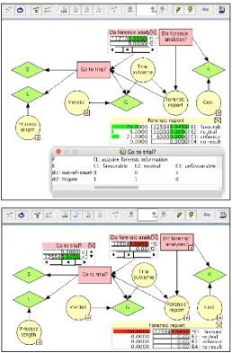
Figure 6: Bayesian decision network previously defined in Figure 4, extended here
with a child node for 𝜃, representing the scope of results E given by a forensic
scientist’s report. Figure (i) shows the initial state of the network with litigation costs
fixed at € 20K and the verdict fixed at € 150K. Figure (ii) shows a situation in which a
forensic report favourable to the defendant is obtained. This is highlighted with a grey
shaded node, instantiated to 𝐸1. The forensic information 𝐸1 leads to posterior
probabilities for the trial outcomes 𝜃 and an EMV of € 125,946 for the optimal decision
𝑑2.
Forensic result E Pr (𝜃1|𝐸𝑖) 𝑑𝑜𝑝𝑡|𝐸 EMV(𝑑𝑜𝑝𝑡|𝐸) EMV(𝑑𝑜𝑝𝑡|𝐸) × Pr(𝐸)
𝐸1(favourable) {0.973,0.027} 𝑑2 € 125,946 € 93,200
𝐸2(neutral) {0.8,0.2} 𝑑2 € 100,000 € 5,000
𝐸3(unfavourable) {0.19,0.81} 𝑑1 € 90,000 € 18,900
Total: € 117,100
Table 1: Illustration of the computation of the EMVpI. For each forensic result 𝐸𝑖,
i={1,2,3}, the columns two to five contain, respectively, the posterior probabilities
{Pr (𝜃1|𝐸𝑖), Pr (𝜃2|𝐸𝑖)}, the a posteriori optimal decision (𝑑𝑜𝑝𝑡), their associated EMV,
and the EMV discounted by the marginal probability of the finding 𝐸𝑖. The total value
in column five gives the EMVpI (Equation (12)).
The direct computational step to obtain the EVpI for the forensic report E
is shown in Figure 7, using the “Value of information” functionality of the
software Hugin. The EVpI can be retrieved in an information pane while keeping
d1: out-of-court
settlement € 90,000
d2: go to trial€100,000
q1: win 0.8
q2: lose 0.2
G L S (i) 100,0000.0 150,000 1.0 200,0000.0 20,000 1.0
40,000 0.0
E1: favourable 0.74
E2: neutral 0.05
E3: unfavourable0.21
d1: out-of-court
settlement € 90,000
d2: go to trial€125,946
q1: win 0.973
q2: lose 0.027
G L S (ii) 100,0000.0 150,000 1.0 200,0000.0 20,000 1.0
40,000 0.0
E1: favourable 1.0
E2: neutral 0.0
track of other key values shown in monitor windows besides nodes in the
network (e.g., EMV of the a priori optimal action, here 𝑑2, which is € 100K).
Figure 7: Illustration of a computerized implementation of the Bayesian decision
network as defined and instantiated in Figure 6(i) (i.e., litigation costs fixed at € 20K
and the verdict settlement fixed at € 150K), using the software Hugin Researcher (vers.
8.6). The information pane shows the result of a value of information analysis for the
decision variable representing the plaintiff’s decision of bringing or not the damage
suit to trial. The result of the analysis, € 117,100, is the EVpI, the expected value of
partial information. Here, partial information refers to the forensic report. It
corresponds to the result obtained in Section 3.6, and is given by the difference
between the EMVpI (that can be found in, or that has been reconstructed step by step
in Table 1) and the EMV of the a priori optimal action (here, € 100K, shown also in the
monitor window of the decision node “Go to trial?”).
3.7 Sequential decision-making and normative decision policies
So far we have considered a formal way of thinking about the value of a single
item of information in the context of making an important decision, illustrated
through the example of a hypothetical litigation case. This analysis can be taken
a step further and be reflected on from the perspective of sequential
decision-making. In the currently discussed example, the decision about whether or not
the damage suit to trial. Thus, there is a sequence of decisions. In terms of a
Bayesian decision network, the decision about obtaining or not forensic
information can be represented by adding an additional decision node, denoted
F here, as a parent for the node E. The values of the node F are “acquire forensic
information (𝑓1)” and “do not acquire forensic information (𝑓2)”. The node F has
a utility node K as a child, in order to account for the cost of the forensic
information. The chance node K′ deals with uncertainty about these costs as done
previously for the nodes G′ and L′. Figure 8 summarises the network. Note that
there are additional edges with dotted lines. One edge is a precedence link and
goes from the decision node F to the decision node D. This indicates the temporal
order that decision F precedes decision D. Another edge, an information link,
goes from E to D. This dotted edge indicates that the state of the variable E is
known before the ultimate decision D is made. These semantic aspects are also
known as the no-forgetting assumption: the decision-maker perfectly recalls all
“experiments” and decisions made in the past.
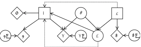
Figure 8: Bayesian decision network previously defined in Figures 4 and 6, extended
here by a decision node F with states “acquire forensic information” (denoted 𝑓1 in the
main body of the text) and “do not acquire forensic information” (denoted 𝑓2). The
utility node K models the cost of acquiring forensic information, whereas the node K′
models different costs in the same way as is done by the nodes G′ and L′.
D q
G L
S
G’
L’ E
F
The definition of the node E has slightly been changed, by adding a further
state called “no result”. It accounts for the situation in which the node F takes the
value “do not acquire forensic information (𝑓2)”. The definition of the conditional probability table for the node E from Section 3.6 is modified to Pr(𝐸𝑖|𝜃1, 𝐹 = 𝑓1) =
{0.9,0.05,0.05,0} and Pr(𝐸𝑖|𝜃2, 𝐹 = 𝑓1) = {0.1,0.05,0.85,0}, for i = 1,2,3,4. In case of
𝐹 = 𝑓2, not acquiring forensic information, we specify Pr(𝐸𝑖|𝐹 = 𝑓2) = {0,0,0,1},
regardless of the state of the node 𝜃.
Implementing the Bayesian decision network shown in Figure 8 in a
graphical modelling software, such as Hugin, allows one to conduct a variety of
analyses. A first important question is: “Should forensic information be
acquired?”. To answer this question, we need the EMV(𝑓1). In Hugin, this value
can be obtained by using the iterative algorithm called “Single Policy Update”.
As shown in Figure 9 (top), the value obtained is 117,000, which corresponds to
the EMVpI found at the end of Section 3.6 (see also Table 1). This value is greater
than the EMV 100,000 for not conducting forensic analyses (not shown in Figure
9). Note that the cost for the forensic analyses has been set to zero here in order
to allow for a direct comparison of the output with the results obtained in Section
3.6.
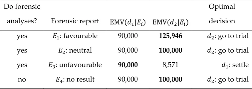
Following the decision to acquire forensic analyses (decision node F), the
next question will be whether or not to bring the case to trial (decision D). This
second decision is considered here to depend on the outcome of the forensic
report. To help with this question, consider again Figure 9 (top). The monitor
window of the node E (“Forensic report”) shows the probabilities for obtaining
the various reports outcomes 𝐸𝑖, for i = 1, ..., 4, as well as the EMV of the optimal terminal decision at the node D (“Go to trial?”). As may be seen, these values
correspond to the EMV(𝑑𝑜𝑝𝑡) obtained in column 4 of Table 1. Note, however,
that the optimal decisions 𝑑𝑜𝑝𝑡 vary: for a favourable (𝐸1) and a neutral (𝐸2)