Published online December 09, 2014 (http://www.sciencepublishinggroup.com/j/ijber) doi: 10.11648/j.ijber.s.2014030601.21
ISSN: 2328-7543 (Print); ISSN: 2328-756X (Online)
Comparison between two types of inventory targets under
variability of a semiconductor supply chain
Kenichi Nakashima
1, *, Thitima Sornmanapong
1, Hans Ehm
2, Geraldine Yachi
21
Department of Industrial Engineering and Management, Kanagawa University, Yokohama, Japan
2
Infineon Technologies AG, Neubiberg, Germany
Email address:
[email protected] (K. Nakashima)
To cite this article:
Kenichi Nakashima, Thitima Sornmanapong, Hans Ehm, Geraldine Yachi. Comparison between Two Types of Inventory Targets under Variability of a Semiconductor Supply Chain. International Journal of Business and Economics Research. Special Issue: Supply Chain Management: Its Theory and Applications. Vol. 3, No. 6-1, 2014, pp. 74-80. doi: 10.11648/j.ijber.s.2014030601.21
Abstract:
As an innovation in the semiconductor industry grows speedy, supply chain processes have not followed up. The variability in semiconductor supply chain have increased and been more complicated. These results in accurately forecast demand and set inventory target. Demand and supply are more and more stochastic and non-stationary. Inventory is one of the methods that companies are able to buffer themselves from complex and variable environment, while still being able to satisfy customer needs. We explore the variability of semiconductor industry in automotive industry. On the supply side, we evaluate variability in complexities of manufacturing process and also products are composed with multiple parts efforts to stochastic production lead-time. However in this paper, we disregard the variability arising from supply side so we assumed lead-time is fixed at 16 weeks. For demand side, the phenomenon is known as the bullwhip effect, the demand variability increases as one move up a supply chain, severely effects to semiconductor supply chain. This results the stochastic demand process is not well understood. Thus we evaluate the stochastic in demand as two aspects: 1) the dispersion of historical demand data from its mean which denoted as standard deviation of demand, 2) the difference between the actual demand and forecast data which denoted as standard deviation of forecast error. We use them as a proxy for demand variability. Then we apply the data to the base stock model. Then, we determine what each variability parameter contributes to inventory. The inventory model represents the semiconductor manufactory’s inventory with actual statistical data which provided from semiconductor company to calculate inventory target required to meet the desired customer service level.Keywords:
Demand Fluctuation, Base Stock Model, Inventory Targets1. Introduction
Automotive industry has been undergoing a change with respect to the implementation of semiconductors into vehicles. Semiconductor technology has enabled many automotive systems manufactures to integrate various applications on a single chip by reducing the board area and optimizing performance. In the automotive semiconductor supply chain, relied upon by 1) several major semiconductor suppliers which we call it as Teir2nd, 2) manufacturers who are responsible for delivery of the finished assembly which we call it as Teir1st, 3) Original Equipment Manufacturer, OEM’s.
The suppliers’ relation in automotive industry has made advance in significant evolution since Just-in-time or Lean production were discovered. The impact to SCM in the automotive industry is an efficient forming relationship with
Teir1st and OEM’s. Since Lean production absolutely relies on suppliers to have the right part at right place and at the right time [3]. Once virtually all companies’ information and knowledge are shared, both Teir1st and OEM’s can have a full understanding to get the job done. Such a close relation between OEM’s and Tier1st has had a substantial impact on Tier2nd. A successful information sharing has not been developed between Tier1st and Tier2nd results in a Tier2nd not being able to response to sudden and unpredictable requirements from Tier1st in EU area.
inventory management. Our analysis of supply chain variability focuses on semiconductor manufacturer in automotive industry.
Figure 1. Automotive Suppliers’ Relations.
The remainder of this paper is organized as follows; section 2 gives a literature review of this research area, then we discuss some factors which give the impacts on an inventory model and analyze the variability in demand parameter in section3. In section 4 the base stock inventory model is described. Section 5 presents numerical results of the simulation inventory model based on the statistical data. Finally, we conclude inn section 6.
2. Previous Works
There are many researches in the field of stochastic inventory management.
Graves and Willems [1] say the safety stock is needed in a manufacturing system due to uncertainties in the requirements, production, and supply processes, and due to the inflexibility of the manufacturing system. They present the first model for a single production stage and the model is a discrete-time model, in which events occur only at the start (or end) of a period. The focus of the research is to decide how much inventory to keep between various production stages in order to provide. To set base stock level demand is an independent identically and normally-distributed random variable with mean µ and variance σ2.
Neale and Willems [9] use the implications of the base-stock model by showing how yield variability can be incorporated in a supply chain facing stochastic, nonstationary demand. Matthew and Willems[6] use the forecast and actual demand history to calculate how the forecast deviates from the actual demand. These data was used for characterize µ and σ for defining the base stock.
Thomopoulos[10] gives a comparison between two fundamental methods of determining the safety stock. The methods are denoted as availability and service Level. The safety stock is the stock carried to meet the uncertainty associated with the forecasts of the demands. The uncertainty
in demands is a measure of the forecast error.
Kojima et al. [4] adapt the kanban contol as one of the most powerful tools in lean manufacturing to a supply chain under stochastic demand and optimize the number of kanbans. Nakashima and Gupta [7] and Nakashima et al. [8] model and analyze disassembly system in the automotive industry using kanban contol systems. The kanban system is well known as the similar to base stock inventory control.
This paper differs from the earlier work in terms of the comparing 2 approach for setting base stock level: 1) using data based on historical demand, 2) using data based on forecasting error. Also this paper investigates the semiconductor’s inventory management when company has a specified forecast accuracy of 70%. In this model, the production order releases are computed based on the forecasted demand adjustments for WIP discrepancy. Adjustments for inventory discrepancy depend on the approach as different types of standard deviation are utilized and desired service level. The rates of adjustments of these discrepancies are identified as the
3. Base Stock Model of Supply Chain
with Variability
In the semiconductor supply chain, the manufacturing organizations have completed variability analyses in order to understand and control process parameter with impact quality.
3.1. Variability Type
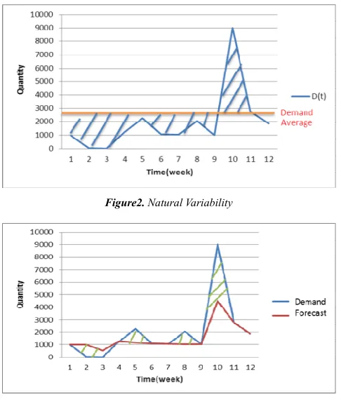
describe natural variability is the standard deviation of the distribution of the historical demand.
3.2.Coefficient of Variation, CV
In the both natural and forecast variability, the relative variability can be calculated by dividing standard deviation by mean value. Since the variability of parameter usually increases in proportion to its mean values, the coefficient of variation, CV is a way to compare across product. By scaling the variability to mean of actual demand, we use these values to model inventory of product with different coefficient of variation, CV from 0.3, 0.5 and 0.7. Low values, 0.3 is associated with stable customer demand, and a higher value, 0.7 is associated with unstable customer demand.
Figure2. Natural Variability
Figure3. Forecast Variability
3.3. Variability Metrics-MPE and SMAPE
There are a significant number of forecast variability measurements. Some result in misleading summary statics. For example, MPE, Mean Percentage Error is an accuracy measure based on percentage errors.
MPE =1/n×
Anyway, result from MPE can be skewed by largepercentage error caused bysmall data scale and an effect of bias (see Appendix A). A measurement which mitigates the effect of outlier and bias is desirable. Symmetric mean absolute percentage error which called SMAPE. With SMAPE1, the forecast bias is divided by the average of forecast and actual demand.
SMAPE1 =1/n×
The formula above provides a result between 0% and 200%. However a percentage error between 0% and 100% is much easier to interpret, then SMAPE2 was introduced. But SMAPE2 favors higher than actual forecast. It is not as symmetric as it sounds since over- and under-forecasts are not treated equally.
SMAPE2 =1/n×
However the MPE and SMAPE1, SMAPE2are vulnerable to
outliers and biases,it is an effective way to use SMAPE3whereby SMAPE3 is more or less protected from outliers and biases.
SMAPE3=
∑
=
−
n
t
t nd Actualdema Forecast
1
) (
/
∑
=
+
n
t
t nd Actualdema Forecast
1
) (
Since SMAPE3 is protected against large errors caused by small scale data and can reduce the problemof upward bias, we use SMAPE3 measurement in our work.
3.4. Variability in Forecasts
The forecast is generated by the industry experts in marketing section who use the combination of economic models, customer forecast, production capacities data, competitive information and intuition for generating forecast for different product. A significant contributor to any forecast error is called bias. Bias represents a consistent forecast error in the same direction (actual sales usually being above forecast or below forecast) over a period of time. The bias can be defined as under-forecasting and over-forecasting. Under-forecasting is a situation where the actual demand exceeds the forecast which we call SMAPE N, N%. Over-forecasting is a situation where actual demand is below the forecast which we call SMAPE P, P%. According to the real data from semiconductor company, it is interesting to note that forecasts for overall product are positively biased in all time horizons as shown below.
We may say that the forecast error is one of the significant parameter for doing business in semiconductor industry. Then we evaluated the variability of forecast error as a measure of the ability of forecast well which showed in figure 5.
Figure 5. The variability of forecast error
The range of CV is from 0.5 to 0.9, we see that forecast are not quite a good demand signal.
3.5 Implication of Variability in Supply Chain
After considering the variability in semiconductor supply chain, it is quite common to say that semiconductor company’s forecasting is bad. This raises the question that company should improve the forecast method to get the better forecasting data. However, to improve forecast accuracy in semiconductor industry is hard. The first reason that why improving forecast accuracy is hard is that there is high demand volatility. The volatility observed in the high-tech markets such as semiconductors often leads tohigh variability in business plan. Second, macroeconomic factors cause the shift in supply chain. This shift is known as the bullwhip effect, where variability gets amplified as the demand signal propagates up the supply chain [3]. Third, short semiconductor product lifecycles have little or no demand history, As a result, planning to customer-driven marketing forecasts was adequate. Forth, there are complex and complicated in the production process, which make supply forecasting required to meet demand is difficult. Sixth, the manufacturing is unable to quickly respond to forecast change due to long production lead time.
As the result of variability in supply chain, our suggestion is to modify the planning system to account for the inherent variability in existing process. The specific suggestion is presented in the next section.
4. Stochastic Inventory Control Problems
In this section, we discuss the stochastic inventory control model which is composed of one production node and one inventory node. This model oversimplifies the supply chain and assumption about the system which may not be perfectly accurate. However this model is more useful than some others model because it was implemented based on actual data about the average lead time or variability parameter. The suggestion resulting from this paper is that deciding the inventory target which can provide the better fill rate where
Fill rate = 1-(quantity of backorder/quantity of actual
demand)
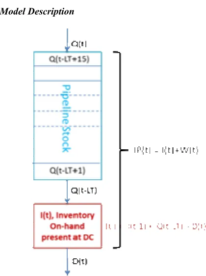
4.1 Model Description
Figure 6. Diagram of Basic Inventory
The primary assumption of model are periodic review, no set up cost, no lot sizing, infinite production capacity and net replenishment lead-time, LT is fix as 16 weeks according to actual data. In a basic inventory model, shown in Figure 6, an inventory is supplied by a production pipeline that has a constant lead time, LT. CQ(0; t] denotes the cumulative quantity of production ordered up to time t, and CD(0; t]
denotes the cumulative demand on the inventory up to time t. In this paper lead time is set as constant value. I(t) means on hand Inventory level at the beginning of period t and is given by the following equation.
I(t) = CQ(0, t -LT] - CD(0, t] (1)
I(t) is allowed o be negative, so demand can be backorder. We will henceforth refer to I(t) as the on-hand inventory.
To proceed further, we need a model of how ordering takes place in response to demand. To define the policy, inventory position is introduced. The inventory position, IP (t), is defined as
IP(t) = I(t) + CQ(t – LT, t] (2)
where CQ(t-LT, t] = CQ(0, t] - CQ(0,t-LT] is the total quantity ordered in the last 1 units of time, which is the total quantity in the pipeline that is due to arrive by time t + LT.
CI(t+ LT) =CQ(t-1, t] -CD(t, t + LT] + I(t) (3)
= P(t) -CD(t, t + LT]
So the on-hand inventory on lead-time in the future is the current inventory position minus the demand between now and time t + l. The term, CD(t, t + LT],is the demand during lead time demand. Note that while P(t)is completely controllable, there is absolutely no control over the demand during lead time demand CD(t, t+ LT]. All that can be done is to control the inventory position, P(t).
4.2. Base Stock Policy
Under this system, total inventory can be calculated to meet desired fill rate, whereas taking into account source of variability, the equation is shown below.
Base Stock Level (BS)
=µd×(LT+r) + Z-1(α)×σd×(LT+r)1/2
where µd= average demand over replenishment lead-time
r= review period
LT= replenishment lead-time
α= service level; probability of (not out of stock during the replenishment lead-time)
Z-1= safety factor calculated from service level σd= variability in demand
The pipeline stock or work in process is represented by the average demand time replenishment lead-time. The average demand time review period represent the cycle stock. In this work, we assume that average demand over review period is equal to production over review period. Thus, cycle stock is not related with analyzed variability, then we take it away from analysis. The last term in the equation refer to safety stock from variability, therefore we will focus on safety stock.
4.3. Safety Stock with Variability Demand
Safety stock is required to buffer from variability over replenishment lead-time. This can be calculated by determining the standard deviation of historical demand or standard deviation of forecast error. Variability in demand can be characterized as
1)Natural Variability; historical demand = 2/n
2)Forecast Variability F/C error= 2/n
To the canonical difference between the two types of variability, the resulted fill rate from the model based on natural variability and forecast variability is monitored, in the aspect of which one is an accurate predictor of future variance in different product.
4.4. Production Quantity Control
It is important for managers to realize that how they run items using production quantity control which has a great impact on inventory. The production quantity should order to
minimize the total inventory costs by balancing production cost, inventory holding cost and penalty cost (back order cost). By definition of adaptive base stock policy, where base stock is reset every month, production quantity, Q(t)is determined by following rule; where the inventory position,
IP(t) in period t after demand fulfillment but before order placement, and D(t) represents the actual demand:
Q(t) = BS(t)– IP(t) (4)
= BS(t) – [BS(t-4) – D(t)]
This production ordering process is called the order up-to model which is a pull system because inventory is ordered in response to demand(Figure 7).
Figure 7. Production Ordering Policy.
5. Computational Results
Here the simulation model was developed based on the base stock model described in section 4 in Excel to simulate the performance of new base stock policy and verify an accurate predictor of future variance proposed in section 4.3.
5.1. Significant Parameters
Control parameter ;α = Service Level (Available)
Condition input parameter ;SMAPE3 = 30%
Condition output parameter; = Fill Rate
where we observe the criteria when 2 options yield the same fill rate
Criteria ; E[I(t)] = Average Inventory On-hand
CV = coefficient of variance of demand
T = time horizon plan
n = repeat time
In this simulation, the time unit is week. The data of forecast accuracy which calculated based on SMAPE3 is based on real semiconductor company.
5.2. Simulate Process
1)Set [75% , 99.99%]
2)Generate n replications of Actual Demand(D) 3)and Forecast(F) (see Appendix B)
4)For each replication, compute the average inventory on-hand and fill rate.
7)Choose the E[I], estimate inventory on-hand level that gives the same E[β], estimated fill rate from each approaches and compare E[I]
8)Run simulate with different product which categorized by difference CV
5.3. Comparison of the Policies
This section presents the result of work done from single stage simulation experiment. First we present the variability in semiconductor supply chain within which to understand the impact of variability on process. With an understanding of variability inherent in the system, we can begin to simplify analyses by using less variability data. Once variability in system has been measure, we will be able to avoid more variable data. Therefore, we compared 2 approach; 1) using data based on historical demand 2) using data based on forecasting error for setting base stock level. We utilized the real data to establish relationships between variability and inventory requirement. Based on the evaluated of data and scenarios, the results of simulation are shown as the following figures.
Figure 8. Better contributor in demand variability, CV of 0.3
For product which has stable demand performance (CV=0.3), forecast error data, forecast variability is used as a proxy for variability. For product which has unstable demand performance (CV=0.7), historical demand data, natural variability is used as a proxy for variability. With this result, company can link related variability to improve the demand-supply system in order to archive the required fill rate (delivery performance). However, this paper needs to develop and extend to be more complexity. Follow-on research should include the development a model to ramp-up period.
Figure 9. Better contributor in demand variability, CV of 0.5.
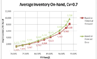
Figure 10. Better contributor in demand variability, CV of 0.7
6. Conclusion
This paper dealt with the stochastic inventory control problem with uncertainty in the supply chain. We compared inventory policies based on the base stock system. We evaluated the stochastic in demand as two aspects: 1) the dispersion of historical demand data from its mean which denoted as standard deviation of demand, 2) the difference between the actual demand and forecast data which denoted as standard deviation of forecast error. We used them as a proxy for demand variability. Numerical results showed the properties of the policies in the different scenarios.
Acknowledgement
This research is supported in part by JSPSGrants-in-Aid for Scientific Research No. 23510193.
Appendix A- Outlier and Bounded in
MAPE, SMAPE
1and SMAPE
2Case 1. MPE is skewed by largepercentage error caused bysmall data scale.
Forecast Actual Demand (Ft-Dt)/Dt
SKU 1 2 4 50%
SKU 2 58 50 16%
SKU 3 50 50 0%
SKU 4 42 50 -16%
SKU 5 48 50 -4%
MPE -11%
MPE (exclude SKU 1)
-1%
MPE and MPE (exclude small data, SKU1) give quite different result.
Case 2. SMAPE1 and SMAPE2are vulnerable to outliers and biases.
Forecast Actual Demand l(Dt-Ft)l / (Dt+Ft)/2 l(Dt-Ft)l / (Dt+Ft)
SKU 1 50 200 120% 60%
SKU 2 50 200 200% 100%
SKU 3 50 150 100% 50%
SKU 4 60 50 18% 9%
SKU 5 40 50 22% 11%
SMAPE 1 92%
SMAPE 2 46%
Appendix B- Generate Demand Data and
Forecast Data Under the Condition of
Having 70% Forecast Accuracy
Calculated by SMAPE3
Table A1. Relationship among the variables
i Di Fi pi lDi-Fil pi(Di-Fi) pi(Di+Fi)
1 x1 f1=ax1 p1 x1- ax1 p1 (a-1) x1 p1 (1+a) x1 2 x2 f2=ax2 p2 x2- ax2 p2 (a-1) x2 p2 (1+a) x2 3 x3 f3=ax3 p3 x3- ax3 p3 (a-1) x3 p3 (1+a) x3 4 x4 f4=ax4 p4 x4- ax4 p4 (a-1) x4 p4 (1+a) x4
5 x5 f5=x5 p5 x5- x5 p5 (0) p5 (0)
6 x6 f6=bx6 p6 x6-bx6 p6 (1- b) x6 p6 (1+b) x6 7 x7 f7=bx7 p7 x7-bx7 p7 (1- b) x7 p7 (1+b) x7 8 x8 f8=bx8 p8 x8-bx8 p8 (1- b) x8 p8 (1+b) x8 9 x9 f9=bx9 p9 x9-bx9 p9 (1- b) x9 p9 (1+b) x9
Let:
Di = demand data Fi= Forecast data
pi = probability x5 = median = mean Analyzing :
i. when the actual demand is lower than its mean, there is a high probability of over-forecast event (Forecast > Actual demand)
ii. when the actual demand is higher than its mean, there is a high probability of under-forecast event (Forecast < Actual demand)
Assuming: Forecast Accuracy = 70%, Over-forecasting = 10%
Equation: At Forecast Accuracy of 70%
E[SMAPE] = E[(∑lD-Fl)/∑(D+F)] = 0.3 (A1)
[(a-1) + (1-b) }/ ] = 0.3
Over-Forecasting = 10%, which means Under-forecast = 20%
{(a-1) / = 0.1 (A2)
{(1-b) }/ = 0.2 (A3)
Generate the demand data from x1to x9, and the forecast data from f1 to f9 where let the x5 is median. Then find a and b from equation 2 and 3.
We can get the following results;
a = 152%
b = 34 %
By scaling the variability to mean of actual demand, we use these values to model inventory of product with different coefficient of variation, CV from 0.3, 0.5 and 0.7, where CV of demand is set as follow CV = Standard Deviation / mean=
[(Di- )2/n]1/2/[∑(Di × pi)/n]
References
[1] S. Graves and Willems S., “Optimizing Strategic Safety Stock Placementin Supply Chains,” Manufacturing & Service Operations Management Vol. 2, No. 1, Winter 2000, 2000, pp. 68–83
[2] G. Guillermo and Garrett J., “Optimal Dynamic Pricing of Inventories with Stochastic Demand over Finite horizons,” Management Science, Vol. 40, No. 8, 1994, pp.999-1019
[3] E. Hans, “The Bullwhip EffectAnylogic Conference Supply Chain Innovation,” Berlin, Germany,AnyLogic Conference 2012, www.anylogic.com/alc-2012
[4] M. Kojima and Nakashima. K and Ohno.K., “Performance Evaluation of SCM in JIT envi-ronment”. International Journal of Production EconomicsVol.115, No.2, 2008, pp 439-443.
[5] F. L. Marshall and Janice H. Hammond., “Making Supply Meet Demand in an Uncertain World,” Harvard Business Review, Vol. 94302, 1994, pp83-93
[6] M.P. Manary and Willems S., “Setting Safety-Stock Targets at Intel in the Presence of Forecast Bias,” Management Science, Vol.38/2, 2008, pp.112–122
[7] K. Nakashima, Kojima M. and S. M. Gupta, “Management of a Disassembly Line using Two Types of Kanbans,” International Journal of Supply Chain Management, Vol.1, No.3, 2012, pp. 11-19.
[8] K. Nakashima, Thitima S. Hans E. and G. Yachi, “Stochastic Inventory Control Systems with Consideration for the Cost Factors Based on EBIT,” International Journal of Supply Chain Management, Vol.3, No.3, 2014, pp. 68-74.
[9] J. Neale and Willems S., Managing Inventory in Supply Chains with Nonstationary Demand, Interfaces Vol. 39, No. 5, 2009, pp. 388–399