M E T H O D O L O G Y
Open Access
BioMiCo: a supervised Bayesian model for
inference of microbial community structure
Mahdi Shafiei
1†, Katherine A Dunn
2†, Eva Boon
2†, Shelley M MacDonald
2, David A Walsh
3, Hong Gu
1and Joseph P Bielawski
1,2*Abstract
Background:Microbiome samples often represent mixtures of communities, where each community is composed of overlapping assemblages of species. Such mixtures are complex, the number of species is huge and abundance information for many species is often sparse. Classical methods have a limited value for identifying complex features within such data.
Results:Here, we describe a novel hierarchical model for Bayesian inference of microbial communities (BioMiCo). The model takes abundance data derived from environmental DNA, and models the composition of each sample by a two-level hierarchy of mixture distributions constrained by Dirichlet priors. BioMiCo is supervised, using known features for samples and appropriate prior constraints to overcome the challenges posed by many variables, sparse data, and large numbers of rare species. The model is trained on a portion of the data, where it learns how assemblages of species are mixed to form communities and how assemblages are related to the known features of each sample. Training yields a model that can predict the features of new samples. We used BioMiCo to build models for three serially sampled datasets and tested their predictive accuracy across different time points. The first model was trained to predict both body site (hand, mouth, and gut) and individual human host. It was able to reliably distinguish these features across different time points. The second was trained on vaginal microbiomes to predict both the Nugent score and individual human host. We found that women having normal and elevated Nugent scores had distinct microbiome structures that persisted over time, with additional structure within women having elevated scores. The third was trained for the purpose of assessing seasonal transitions in a coastal bacterial community. Application of this model to a high-resolution time series permitted us to track the rate and time of community succession and accurately predict known ecosystem-level events.
Conclusion:BioMiCo provides a framework for learning the structure of microbial communities and for making predictions based on microbial assemblages. By training on carefully chosen features (abiotic or biotic), BioMiCo can be used to understand and predict transitions between complex communities composed of hundreds of microbial species.
Keywords:Microbial community structure, Bayesian model, Admixture model, Hierarchical mixed-membership model, Supervised learning, OTU abundance data, Microbiome, Human, Temperate coastal ocean
Background
Microbial communities are highly complex assemblages of individual organisms. Hundreds, and sometimes thousands, of species can contribute to a community (for example, [1,2]), with the individuals belonging to a species having a
wide range of interactions with other individuals in that community [3]. Moreover, the species within a community can be structured hierarchically into assemblages. For ex-ample, among all species that contribute to the human gut microbiome, only a subset have stable co-occurrence rela-tionships, with only a further subset seeming to have stabil-ity over decades [4]. Although single species, or strains, have been successfully targeted as causative agents of dis-ease (for example, [5]), there is growing interest to learn how the broader composition of a community might be re-lated to some feature of concern (for example, an
* Correspondence:[email protected] †Equal contributors
1Department of Mathematics and Statistics, Dalhousie University, Halifax, NS,
Canada
2Department of Biology, Dalhousie University, Halifax, NS, Canada
Full list of author information is available at the end of the article
ecosystem process [6], the severity of a disease state [7], the impact of a dietary intervention [8], or source tracking [9]). In settings where community-level function is thought to be important, the co-occurrence relationships among line-ages may be more informative than the simple presence or absence of one, or a few, indicator species [10]. Although sampling community composition via high-throughput amplicon sequencing, or via shotgun metagenomics, is no longer methodologically challenging, the data still pose a significant analytical challenge. Associations within such data are complex, the number of variables is huge, and spe-cies abundance information is sparse for many spespe-cies (or strains) over many samples. In this setting, classic testing procedures have limited ability to identify complex features within the data [11,12].
Statistical model-based supervised learning is ideally suited to the challenges posed by microbial community data. This family of techniques is designed to learn the variables of a model most suited to discriminating among user-defined features of interest. Especially rele-vant to microbial community data is their capacity for (i) learning from very high-dimensional data and (ii) quan-tifying the accuracy of a model at predicting the features of concern in future datasets [11]. Despite these advan-tages, the existing techniques have only recently been applied to microbial community data, and very little de-velopment has been done purposely for microbial com-munity data (but see [9,13]). Readers are referred to Knights et al. [12] for a thorough review of how the standard techniques can be applied to microbial com-munity data.
Here, we focus on the task of building and evaluating a predictive model for microbiome composition data. Taking clinical microbiomics as an example, a typical re-search goal might be to learn how microbiome structure relates to, say, the probability of disease, and then to use that information to monitor and make predictions about an individual’s chance of disease according to his/her own microbiome samples. As a community structure is characterized by the contribution of species to assem-blages, and assemblages to communities, we focus on modeling the relative abundance of both assemblages and species. Hereafter, species are defined operationally according to a sequence similarity threshold (typically 97% for 16S rRNA sequences) and are referred to as op-erational taxonomic units (OTUs) rather than species. Modeling compositional data within a supervised frame-work is not new (for example, [14]), but only two ap-proaches have been developed purposely for modeling relative abundances of OTUs [9,13]. Both Knightset al. [9] and Holmes et al. [13] model OTU abundances by applying a Dirichlet prior to the parameters of the multi-nomial distribution. Knights et al. [9] developed their model for predicting how microbial contaminants might
be mixed within a given sample (that is, source tracking). Their model learns the OTU composition for each of a fixed number of source communities, where all samples for a given source must share a single mixture of OTUs, and then uses this information to predict how much each source might contaminate a given test sample. Holmes et al. [13] employed an approach similar to la-tent Dirichlet allocation (LDA) to model microbiome composition. Their model relaxes the assumption that, when learning about a microbiome structure, all samples for a given feature will share a single mixture of OTUs. However, their model does not provide a means of asses-sing the structure of the microbiome in terms of readily interpretable parts. In this study, we describe a novel model (called Bayesian inference of microbial communi-ties (BioMiCo)) that is intended to facilitate interpret-ation of a community structure in light of user-defined feature labels. Ours is a hierarchical model that can be used to simultaneously learn how assemblages of OTUs contribute to microbiome structure and how multiple assemblages might be related to the known features of the samples.
We use these data to illustrate how BioMiCo can be employed to investigate community structure with respect to specific features of interest, and we explicitly evaluate the accuracy of the model to make predictions at different points in time.
Methods
Overview of the analytical framework
We assume that each sample contains information about the abundance of microorganisms within the sampled environment, which will typically be derived from en-vironmental DNA (16S or whole genome sequencing (WGS)). Microorganisms within a sample are expected to show a range of interactions, from very little inter-dependence to obligate symbiosis [3]. Here, we refer to a set of co-occurring OTUs resolved by the model as an assemblage, where the ecological interactions among the members of the assemblage are treated as unknown. However, the microbial associations that are detected with the model can be the starting points for detecting ecological interactions. Indeed, the most direct test for microbial interactions is to experimentally disturb the microbiota and assess the recovery of the same pattern of OTU associations as originally resolved by the model. We follow Boon et al. [3] by using the term community to refer to a collection of OTUs that are explicitly as-sumed, or known, to have a high degree of ecological interaction.
Inference about assemblages under BioMiCo can be based on taxonomic units such as OTUs or on func-tional units such as the Kyoto Encyclopedia of Genes and Genomes (KEGG) Orthology numbers. In all three datasets used in this study, we modeled microbiome structure as statistical mixtures of OTU assemblages. The model can then be used to explain any factor label in terms of several assemblages. Factor labels used in this study included the identity of a human host (for hu-man gut microbiomes), Nugent score (for huhu-man vaginal microbiomes), and season of the year (for a coastal mar-ine microbiome). In many settings, the factor labels are chosen because they are believed to indicate some de-gree of microbial community structure or function. The idea that communities are composed of partially over-lapping assemblages of organisms having variable types of ecological interaction is not new to ecology [15] or to microbiology [16,17]. However, this model is the first to offer a probabilistic framework to discern their structural components according to environmental DNA.
Microbiome samples often represent mixtures of dif-ferent microbial communities. Sometimes, this is be-cause it is more convenient to sample mixtures (for example, stool samples are comprised of mixtures of epi-thelium and luminal niche communities [18], but they are much more easily obtained than epithelial biopsies).
Sometimes, samples will be mixtures of communities be-cause we simply do not have sufficient knowledge to precisely target the community of interest (for example, at certain times of the year, a marine community might be stratified or mixed depending on a variety of physical and chemical factors [19]). Because we cannot assume that microbiome samples will always correspond to a single community, we consider each sample as a poten-tial mixture of OTUs from one or more communities. In some cases, it is even desirable to collect and train on samples that represent communities that are mixed to different degrees. Consider the possibility that a differ-ence in microbiome metabolic function could contribute to the intensity of a disease phenotype. In such cases, by training on samples having various mixtures of different communities, the model can learn if a patient’s health status might depend on the degree to which functional and dysfunctional microbial communities contribute to his/her personal microbiome.
The model is supervised, using a portion of the data reserved for “training” to learn which assemblages are associated with a set of pre-selected features of interest. Within BioMiCo, features of interest are called “factor labels,”and the specific value for a given sample is called a“factor value.”Labels can represent generalized factors of interest (for example, season of the year, ethnicity, health status) or specific attributes of a sample (for ex-ample, the identity of the human host in serially sampled data). Users can specify values for multiple factor labels for a single sample by providing unique indicator vari-ables for values coming from more than one label. The training set of samples is used to learn the mixture weights for both (i) the mixing of OTUs within assem-blages and (ii) the mixing of assemblages within samples according to factor values shared across multiple sam-ples. The remaining samples are called the “test set.” Based on the mixture weights learned from the training samples, we compute the posterior probability that a test sample originated from a microbiome having any of the factor values that the model was trained on. If discrete assignment according to factor values is desired, each test sample can then be classified according to the max-imum posterior probability. Since in this study the true label value for each test sample is known, accuracy is measured as the percent of the factor values that are correctly predicted for test samples.
BioMiCo: a hierarchical mixed-membership model
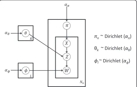
the relative importance of the factors is permitted to dif-fer between samples. The relative contribution of each factor to the nth sample is modeled through the latent variableπn. Furthermore, we only require that some sub-set of this sub-set of known factors is contributing to a given sample. This is different from assuming that every sam-ple is a mixture from all the factors of interest. If this sample can be assumed,a priori, to reflect the contribu-tion of as many as, say, four factors, then πnis a prob-ability vector of four non-zero values summing to one. The probability values for all other non-contributing factors are set to zero. Because we will not know the community structure of the sample, the πnvariables are inferred from the data. We assume a symmetric Dirichlet prior onπn:
πn∼Dirichletð Þαπ
A symmetric Dirichlet is appropriate because we have no prior preference for any of the factors.
Next, we assume that the OTUs that characterize a factor are comprised of a fixed number of OTU assem-blages (L). Therefore, the model differentiates factors ac-cording to their unique mixture of assemblages. The mixture for the kth factor is modeled by a vector of L
mixing probabilities, θk, that sum to one. Thus, there will be K vectors of L mixing probability values. The element θkl in aK×L matrix,θ, represents the relative contribution of assemblage l to factor k. We assume a symmetric Dirichlet prior on rows of θbecause we have no prior knowledge to favor particular assemblages:
θkeDirichletð Þαθ fork¼1⋯K
Finally, we assume that each assemblage is comprised of a mixture of T different OTUs. The contribution of different OTUs to the lth assemblage is modeled by a vector of T mixing probabilities, ϕl, with values sum-ming to one. GivenL assemblages, there will beL prob-ability vectors of length T representing OTU mixing probabilities. Thus, elementϕliin anL×Tmatrixϕ rep-resents the relative contribution of OTUiin assemblage
l. We also assume symmetric Dirichlet prior on rows ofϕ:
ϕl∼Dirichlet αϕ for l ¼ 1 ⋯ L
We use symmetric Dirichlet because we have no prior knowledge to favor a particular OTU in an assemblage. Thus, the model is used to differentiate assemblages ac-cording to their unique mixture OTUs. A plate diagram of the model is shown in Figure 1.
Model inference
The model is used to learn the mixing of OTUs within assemblages and the mixing of assemblages that
characterize a factor value. Let the factor and assem-blage assignments for OTUiin samplenbe denoted by
XniandZni, respectively. Note thatZniis a value between one and L (number of assemblages) and Xni is a value between one andK(number of factors).Wniis the OTU
iin samplenand has a value between one andT. For in-ference, we integrate out all other latent variables and sample from the posterior distribution of the assemblage and factor assignments (Z and X) for each OTU given the data. We use collapsed Gibbs sampling [20] for pos-terior inference. Given a set of variables, in each state of the Markov chain, some (one or more) variables are sampled conditioned on the current values of all other variables and the data in some order.
The complete likelihood of the data given the hyper-parameters of the prior distributions in our model can be written as follows:
P W ;Z;X;ϕ;θ;π α ϕ;αθ;απÞ ¼
P W Z; ϕÞP Z X; θÞP X πÞPϕ α ϕÞPðθ αj θÞPðπ αj πÞ ¼
YN
n¼1 YNn
i¼1
P WnijϕZni
Y
N
n¼1 YNn
i¼1
YN
n¼1 YNn
i¼1
P X niπnÞPϕ α ϕÞPðθ αj θÞPðπ αj πÞ
whereZ, X, θ,ϕ, πare the set of latent variables in our model, Nis the number of samples in a dataset, andNn is the number of OTUs in samplen. For posterior infer-ence, we want to sample from the posterior distribution of latent variables given the data:
P Z ;X;θ;ϕ;πW;αϕ;απ;αθÞ
Because we are interested in sampling from the assem-blage (Z) and factor (X) assignments for each OTU given the data, we integrate out the other latent variables (θ, ϕ, π) and sample from the posterior distributions of
Z and X, or P(Z, X|W, αϕ, απ, αθ). This posterior distribution can be derived analytically for our model [see Additional file 1]. We use Gibbs sampling for drawing samples from this distribution.
At each iteration of the Gibbs sampling, we repeat the following in a random order. For each OTU in each sample, we draw the assemblage and factor assignment (ZniandXni, respectively) of this OTU given the current assemblage and factor assignments of all other OTUs in this and every other sample. Let Z−ni represent the as-semblage assignment for all OTUs in all samples except only OTUiin microbiome sample n. And, letX−ni rep-resent the factor assignment for all OTUs in all samples except only OTUiin microbiome samplen. Each of the individual terms for the conditional distribution can be analytically derived:
P Xni ¼k;Zni¼l X −ni;Z−ni;W;αϕ;απ;αθÞ ¼
Cwnil þ αφ X
w; Cw0nil þ αφ
Ckl þ αθ
X
l0 Ckl0 þ αθ
XCnk þ απ k;ðCnk0 þ απÞ
whereCwnil is the number of times OTUiin samplenis
drawn from assemblagel. Cklis the number of times an OTU is drawn from assemblagel contributing to factor
k. Cnk is the number of times an OTU in sample n is drawn from factor k. Solutions for the individual terms of the conditional distribution are provided in Additional file 1. From the above equation, a value is calculated for each possible combination of values forXniandZni. Note that Xni can take only factor assignments that are known to be contributing to samplen. These values are then normalized and used to draw new assignment values for Xni and Zni which are immediately updated for use in the next iteration. In this study, we also employed a Metropolis-within-Gibbs sampling scheme to learn the hyper-parameters (αθ,αϕ, and απ) from the
data. Metropolis-Hastings updates were used to resample new values for hyper-parameters once all the other param-eters of the model have been sampled. Analyses of all datasets were initialized with hyper-parameter values of 0.01. In this study, the first 200 iterations of the Markov chain Monte Carlo (MCMC) for the training phase were considered “burn-in” and were discarded. Following the burn-in, the MCMC was run for a minimum of 2,000 iter-ations, and samples were retained every 100 iterations. Chains were run multiple times, and if the posterior distri-bution of assemblages was not concordant among runs, the chains were run longer.
Predicting the contribution of different factors to an unlabeled sample
This model can be used to predict the factor values for a sample for which we do not have factor assignments. Labels are chosen by the user, and they can represent specific factors of interest (for example, healthy vs. dis-eased state) or, more generally, the physical aspects of an environment (for example, different concentrations of a limiting nutrient). The model is first trained on data where each sample is assigned to a possibly distinct known subset from the set of all available factors. The trained model is then applied to test data topredict fac-tor contributions for each sample. Known features of samples can be intentionally hidden from the model for the purpose of testing its performance.
We want to sample the posterior distribution of factor assignments given the OTU distribution of the test data by using what the model has learned from the training data; that is, P(Xtest|Xtrain, Ztrain, W, αϕ, απ, αθ). To
achieve this, we sample from posterior distribution of
Xtest and Ztest jointly, that is, P(Xtest, Ztest|Xtrain,
Ztrain, W, αϕ, απ, αθ), and marginalize over the
assem-blage assignments to obtain the posterior probability of each factor assignment. In this analytical phase (testing), Gibbs sampling is very similar to the training process. The difference is that we do not need to iterate over the samples in the training set; we carry forward the count variables Cwnil and Ckl from the training phase, and we
do not need to run the MCMC for as many iterations. The first 50 iterations of the testing phase were dis-carded as “burn-in,” and the MCMC was run for an additional 1,000 iterations with samples retained every 50 iterations. In all datasets examined in this study, the number of factor labels (K) is determined by the re-search question, and the number of assemblages (L) was set to 100.
Implementation
available at http://sourceforge.net/projects/biomico. Being a generative model, we simulated a microbiome sample for the purpose of testing the inference algorithm. See Additional file 2 for an overview of the generating process. We simulated data over a very wide range of conditions (504 scenarios, each comprised of 200 microbiome sam-ples) and used it to (i) verify that our training phase can recover the parameter values used to generate structured microbiome and (ii) investigate what conditions represent easy and hard inference problems for the testing phase. Results confirmed the reliability of the inference algorithm in the training phase and demonstrated that reliable infer-ence of factor labels is possible over a very wide range of conditions. Additional file 2 contains a full description of the simulation design and presents the outcomes of the simulation study.
Results and Discussion
Dataset 1: assessing temporally stable microbial assemblages within the human microbiome
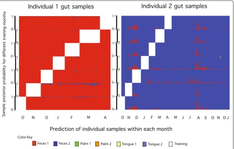
We applied our mixture modeling approach to a detailed investigation of temporal microbiome variation, which entailed long-term sampling of two human individuals at four body sites (gut, tongue, right and left palm) over 396 time points [1]. As both individuals in this study were healthy, there were no clinically significant factors to train on. Although temporally stable strains have been detected within other longitudinal studies of the human gut [4,21,22], temporal stability could not be detected in this study [1]. This makes the Caporasoet al.[1] dataset an especially rigorous test of our approach, which treats OTUs as potential members of assemblages rather than as independent units of diversity. By combining informa-tion from many OTUs within an assemblage (including OTUs having low abundances), we anticipate improved power to detect a temporally stable signature in those data. Further, by training over a small time period (for example, 1 month) and testing the provenance of the samples taken at other times, we can measure the reli-ability of predictions made according to assemblage in-formation for a long window of time.
The original set of OTU counts generated by Caporaso
et al. [1] was filtered to remove all singletons (that is, OTUs observed in only one sample). Our model can be run on data that includes singletons, but they were ex-cluded because they increase computational costs with-out providing a useful signal (and could potentially dilute signal strength for the assemblage membership of other OTUs). Filtering yielded a matrix of 1,967 samples (rows) having 15,685 OTUs (columns). This matrix rep-resented the samples obtained from 396 time points for two human hosts over four body sites; each sample was labeled according to both host and body site (thus, K= 2 × 4 = 8 in this model). As was already reported [1], we
found pronounced variability in microbiota from both subjects across months, weeks, and even days. Also, like the original study, samples from different body sites were easily distinguished throughout the sampling inter-val (Figure 2 and Additional file 3). However, we also uncovered evidence of a hierarchal structure in the form of assemblages of OTUs; the values of both αϕ and αθ
estimated by using Metropolis-Hastings when training on seven different months were substantially less than 1.0 (αϕ: mean = 0.006, min = 0.005, max = 0.007; αθ:
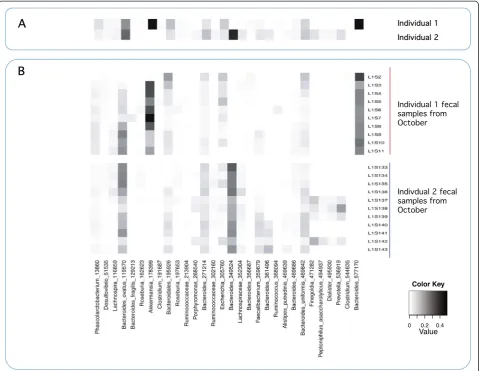
mean = 0.021, min = 0.012, max = 0.026). Further, the mixture weights revealed (i) some OTUs had similar, and temporally stable, mixture weights in both individ-uals (for example,Bacteriodes ovatus119570 in Figure 3), (ii) some OTUs had consistently different mixture weights between individuals (for example, Bacteriodes
577170 in Figure 3), and (iii) most OTUs had no temporal stability. For this dataset, assemblages are composed of OTUs that tend to have the same co-occurrence pattern across serially sampled microbiomes; thus, they can represent a temporally stable signature within these data. Figure 3A shows OTUs from assem-blages that are characteristic of fecal samples from indi-viduals 1 and 2; note that they are composed of OTUs with varying degrees of abundance yet follow the same co-occurrence pattern.
Because the individual-specific mixture weights (that is, patterniiabove) represent a central tendency in OTU composition within the human microbiota, this signal could serve as the basis for making predictions through time. To test the accuracy of a prediction based on such a signal, we attempted to predict the most comprehen-sive feature of a sample, the identity of the human host, based on mixing probabilities learned from samples taken weeks and even months earlier. This approach yielded very high-classification accuracy when using the signal contained within the gut (97%) and the tongue (87%) microbiomes. The signal persists over the full dur-ation of the study. Re-training on different months yielded accuracy between 98.6% and 99.3% when using gut samples and 85% to 93% when using tongue sam-ples. Prediction was more challenging when using the signal contained within palm samples (40% to 75% ac-curacy over the study). However, samples from the hu-man palm pose a special challenge because they are exposed to a wide range of microbial environments over days, weeks, and years.
mislabeled and were excluded from the original study [1]. Exclusion of the mislabeled samples from our study and retraining did not substantially alter classification accuracy. This illustrates that our modeling framework is powerful, even when labeling errors are included in the training set [see Additional file 4].
Some OTUs within the gut microbiome appear to be highly discriminatory; that is, they have a high abun-dance in one individual and a low abunabun-dance in the other. To test that the model is using the co-occurrence information of the OTUs in an assemblage, and not just the frequency differences of those few high-abundance OTUs in the gut, we removed the OTUs with an average relative abundance of greater than 1% in the fecal sam-ples (by setting the raw counts to zero for those OTUs in the fecal test data), and we re-predicted each sample’s host. This led to the exclusion of 14 OTUs from individ-ual 1 and 16 OTUs from individindivid-ual 2. In those cases where testing was possible, classification accuracy was between 81% and 100%. There were two sets of training data where testing was not possible because in those 2 months (October and November) the training data for individual 1 was completely dominated by the 14 OTUs
removed; thus, there was no basis for classification of indi-vidual 1 according to those training data. These results in-dicate that co-occurrence information for low-abundance OTUs contributes to the ability to make predictions at dif-ferent time points.
Recall that previous studies were unable to detect any temporal stability within these data. In contrast, we found that some OTUs maintained host-specific co-occurrence patterns in the face of dramatic temporal variation in community composition. Our focus on as-semblages (which includes the low-abundance OTUs), and our implementation of a supervised framework, made this possible. Note that we do not anticipate that our model will normally be used to identify hosts within serially sampled datasets, as they will be known with cer-tainty. We also expect that sampling additional human hosts will likely reveal some sharing of assemblages (for example, among family members). Our results, however, indicate that (i) there exists temporally stable assem-blages within human-associated communities and (ii) re-liable predictions can be made at future time points according to information about microbial assemblages obtained from training data. If links can be made
between microbial assemblages and status labels for hu-man health (for example, obese, frail, Crohn’s disease, re-mission), the value of microbiomics to personalized healthcare might be further enhanced.
Dataset 2: assessing microbial communities in women with no symptoms of bacterial vaginosis and high Nugent scores
Bacterial vaginosis (BV) is a condition that predisposes women to greater risk of sexually transmitted disease and adverse pregnancy outcomes [23,24]. Nugent et al. [25] described a method of scoring a vaginal smear ac-cording to the relative abundance of selected microbial lineages, and this score is commonly used in research settings to indicate BV. A score between 7 and 10 is considered indicative of bacterial vaginosis, although a
score ≥4 in conjunction with “bacteria covered” clue cells within the smear is also considered consistent with BV. Based on a comprehensive study of temporal dy-namics in vaginal microbiomes of asymptomatic women, Gajer et al. [26] suggested that the notion of a healthy vaginal microbiome might need to be expanded to in-clude the possibility of high Nugent scores. Some women’s Nugent score varied substantially over the course of their study, while others had a long-term ten-dency to score high; yet none of the women reported any symptoms of BV. Given these temporal dynamics, we wanted to determine if our model could identify a community signature consistent with elevated Nugent scores in asymptomatic women. We also wanted to in-vestigate the possibility of additional structure; that is, that there might be some temporally stable differences
among women who persistently score high on the Nugent scale.
We applied our modeling framework to the data of Gajer et al. [26], which was collected twice weekly from 32 reproductive-age women over a 16-week period. As menses can have a dramatic impact on the vaginal community [26], we excluded samples taken during menses. We also excluded samples for which there was no Nugent score. This yielded a matrix of 715 samples (rows) having 330 OTUs (columns). We used a common scheme for discretizing Nugent scores [25,26] and assigned all samples to one of two categories: “normal” (low score: 0 to 3) and“elevated” (intermediate score: 4 to 6; high score: 7 to 10) Nugent scores. Thus, for this model, K= 2. We then randomly assigned two thirds of the samples in each category to a training set and trained the model on those data. The remaining one third of the samples was used to test the accuracy of using OTU co-occurrence patterns to predict an elevated Nugent score. This procedure was replicated five times.
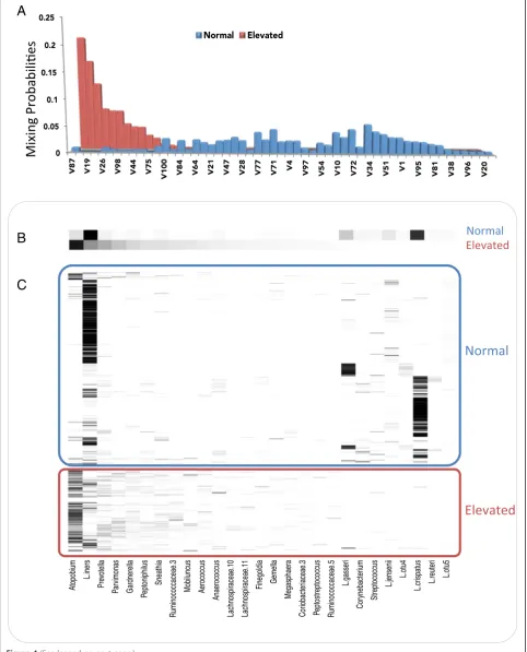
Figure 4 summarizes the structure of the assemblages learned by the model and their mixing probabilities with respect to “normal” and “elevated” Nugent scores. The difference between assemblage distributions (Figure 4A) is due to differences in the depth of community struc-ture. The group of individuals having a“normal”Nugent score had a relatively flattened distribution of highly sparse assemblages. Sparse assemblages are character-ized by just a very few (in this case one to three) OTUs with non-trivial mixing probabilities. The flat assemblage distribution reflects the contribution of many low-abundance OTUs to the “normal” label, as well as the tendency ofLactobacillus inersand Lactobacillus crispa-tus to co-occur with different low-abundance OTUs in different individuals. The group of individuals having “elevated” Nugent scores had a deeper community structure, that is, more complex co-occurrence patterns concentrated in fewer assemblages, yielding a much more skewed assemblage distribution. As the Nugent score is based on the premise that Lactobacilli decrease the score, and that Gardnerella or Bacteroides spp. or curved gram variable rods increase the score, it is not surprising that this signal is contained in the OTU as-semblages (Figure 4). However, the OTU composition of the assemblages with the highest mixing probabilities provides additional information about individuals with elevated Nugent scores; they represent the central ten-dency of co-occurrence relationships over all the train-ing samples havtrain-ing an “elevated” Nugent score. To the extent that these patterns have temporal stability, they can be used to make predictions about unlabeled data.
Patterns of OTU co-occurrence were informative for making predictions about the test data. Mean
classification accuracy over the five random assignments of microbiome samples to the training partitions was 90% (range: 88% to 93%). Interestingly, a large fraction of classification errors were associated with outlier Nugent scores; these are cases where an individual has a consistent time series of “elevated” or “normal” Nugent scores with a single outlier score within this time series. Approximately 50% of the misclassification errors were for this type of outlier; thus, overall classification is im-proved when we attempted to predict an individual’s me-dian Nugent score (92% accuracy; range: 90% to 95%) rather than their sample-specific scores. Note that pre-diction of median scores for seven individuals was a little less accurate than their sample-specific predictions. Re-markably, the prediction of sample-specific Nugent scores was reliable when an individual switched Nugent score categories as long as that switch persisted for a few samples. As the model does not explicitly include temporal autocorrelation, this finding hints at potentially interesting lurking variables that influence microbiome stability over different time scales.
We also investigated if predictions for these data exploited the assemblage information and not just the frequency differences of a few high-abundance OTUs. We removed the OTUs having >1% contribution to the vaginal microbiome samples. This led to the exclusion of seven OTUs from the “normal” score category and 11 OTUs from the “elevated” score category. Classification based on just the low-abundance OTUs was largely un-affected by this data reduction; mean accuracy remained at 90% (range: 89% to 93%). These results verify that the model was able to capture community-wide signatures associated with elevated Nugent scores. To obtain a Nugent score, an experienced microbiologist must assess bacterial cell morphology within a pap smear; we suggest that moving toward an OTU-derived scoring system could mitigate this difficulty. Further, by training on add-itional variables, model-derived scoring systems could be developed for more narrowly defined features of interest. Next, we investigated the possibility of community di-versity among individuals within the group of asymp-tomatic women with elevated Nugent scores. We used two analytical approaches. First, we simply restricted our analyses to the ten women having a median Nugent score ≥4 and tested for individual specific OTU assem-blages (K= 10). Second, we trained a model on the full data where each sample was labeled with respect to both the Nugent score category and the host identity. In this design, the maximum value of K= 2 × 32 = 64; however,
A
B
C
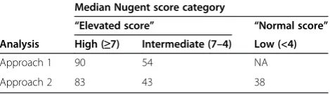
test set. We achieved a remarkably high accuracy (>83%) in predicting the provenance of those samples collected from individuals having a median Nugent score ≥7 (Table 1). We had only moderate success at predicting host provenance given intermediate Nugent scores and even less for individuals having low Nugent scores (Table 1). These results indicate that women with the highest Nugent scores harbored additional microbial as-semblages, and these differences had a remarkable de-gree of temporal stability over the course of the study. This suggests directions for future research. Again, we do not expect that future studies will typically train a model according to individual host identity. We do sug-gest that temporally stable differences among women with high Nugent scores could be related to long-term differences in their status (for example, some women might remain asymptomatic, others might experience limited clinical symptoms, and others might develop re-current BV). By combining longitudinal studies of both asymptotic and BV cases (for example, [27]), and train-ing on additional factor labels (pH, discharge, clue cells, persistent BV, remission, relapse), supervised analyses under BioMiCo could lead to a more refined under-standing of the relationship between community struc-ture and an individual’s manifestation of BV. BioMiCo is not intended as a substitute for other statistical methods [11,28]; rather, it should be viewed as complementary to the methods which are already used to investigate
community structure and track their changes over time (for example, [26,29]).
Dataset 3: assessing seasonality in coastal ocean bacterial communities
Bacterial communities in the ocean are highly diverse [30] and variable across space and time [19,31]. Since com-munity variability is often associated with changes in ecosystem-level processes, the identification of assem-blages of possibly interacting bacterial taxa - and the de-scription of how these assemblages change in time - can contribute to our understanding of how marine ecosys-tems respond to environmental change. The detection of time-dependent co-occurrence patterns among microbial OTUs has been widely employed in time-series studies of marine microbial communities [32]. These studies have shown that ocean bacterial communities exhibit repeating patterns such as seasonal succession and annual reassem-bly [33], and that seasonality can often be linked to envir-onmental conditions and resource availability [2,34]. Given these temporal dynamics, we aimed to determine if our model could be applied to ocean time-series data to iden-tify community assemblages that are characteristic of dif-ferent seasons. Once trained, we also wanted to investigate whether or not the predictive component of the model could provide insight into when and how rapidly bacterio-plankton community succession occurs in the ocean.
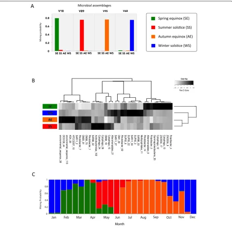
As proof of principle, we applied our modeling frame-work to the data of El-Swais et al. [35], which consisted of a set of OTUs from bacterial communities in the Bedford Basin, a coastal inlet of the temperate northwest Atlantic Ocean sampled over a 6-year period. We trained the model on 24 samples collected from 2005 to 2010; each sample was labeled according to four distinct seasonal time points (thus,K= 4 in this model). The fac-tor values for training consisted of the spring equinox (SE), summer solstice (SS), autumn equinox (AE), and winter solstice (WS). The training phase identified four highly informative assemblages, each contributing a high posterior mixing probability to one of the four seasons (Figure 5A). Hence, as expected, samples from different seasons were clearly distinguishable from each other. More interestingly, seasonal differences in the mixing (See figure on previous page.)
Figure 4Posterior distribution and composition of microbial assemblages with respect to“normal”and“elevated”Nugent scores in asymptomatic human females.Distributions were inferred from the vaginal microbiomes of 32 individuals collected over a 16-week period [26].
(A)Mixing probabilities for the assemblages comprising 95% of the posterior distribution for“normal”and“elevated”Nugent scores.“Normal” was defined by a Nugent score of 0 to 3, and 47 assemblages were responsible for 95% of their posterior distribution.“Elevated”was defined by a Nugent score >4, and 12 assemblages were responsible for 95% of their posterior distribution. As five assemblages were shared between these two distributions, there are a total of 54 assemblages in this plot.(B)Relative magnitude of the mixing probabilities of 27 OTUs (identity is indicated along thex-axis of part(C)marginalized over the 54 assemblages in part(A). Note that 14 OTUs accounted for 95% of the posterior density (PD) of the
“normal”Nugent score category and 19 OTUs accounted for 95% of the PD of the“elevated”Nugent score category. As six OTUs were shared between these two distributions, there are mixing probabilities for a total of 27 unique OTUs in this plot.(C)Empirical relative abundance of the 27 OTUs in the 484 training samples. OTU identity is given along thex-axis. Each row represents an individual sample.
Table 1 Percent correct classification of host provenance according to assemblages in the vaginal microbiomes of asymptomatic women
Median Nugent score category
“Elevated score” “Normal score”
Analysis High (≥7) Intermediate (7–4) Low (<4)
Approach 1 90 54 NA
Approach 2 83 43 38
probabilities of OTUs revealed putative patterns of eco-logical interaction between taxa. A number of OTUs had high-mixture weights for only one assemblage, which is indicative of seasonal specificity. For example,
Polaribacter,Cytophaga, and Alteromonadales OTUs were important members of the SE assemblage (Figure 4B),
which supports earlier studies reporting that these taxa are often associated with the consumption of organic matter from spring phytoplankton blooms [36,37]. Dur-ing the summer, the Bedford Basin surface waters are characterized by low-nutrient availability [38]. As such, it follows that OTUs from the SAR11 and SAR86 clades
were principal members of the SS assemblage (Figure 4B), in agreement with the known oligotrophic nature of these marine bacteria [39,40]. These results demonstrate that even with only a few training samples (six per each sea-son), the model can identify ecological structure in the data. Readers should consult El-Swais et al. [35] for add-itional details about the temporal variability of bacteria in the Bedford Basin.
Once the model training was complete and the sea-sonal assemblages identified, we tested how well the model predicted an additional 25 samples collected at biweekly intervals in 2009. The transitions between as-semblages observed within these data, as inferred by the temporal changes in the mixing probabilities, reflected the seasonal cycle of community succession in 2009 (Figure 4C). Most intriguingly, the timing of the mixing probability transitions, and the time span that a certain assemblage contributed to a sample over the year, was strongly linked to certain events known to occur in the Bedford Basin. For example, a shift from a winter assem-blage to a dominant spring assemassem-blage occurred in early February, which corresponded with the onset of the spring phytoplankton bloom [35]. The spring assemblage continued to dominate through to the end of April, which marked the end of the spring bloom, and was then succeeded by the summer assemblage. In these cases, the model accurately predicted the timing of known ecosystem-level events based on the OTU com-position of samples. However, the model also provided additional insight into bacterial dynamics in the ocean. A clear example of this is the“return”of the autumn as-semblage in late November, which was a striking obser-vation since we expected a steady transition from the autumn assemblage to the winter assemblage from October through December. As it turns out, a short phytoplankton bloom occurred in November, and the re-turn of the autumn assemblage is presumably a response in the bacterial community to this episodic event. Col-lectively, these results demonstrate how a predictive model can be used to track the rate and timing of com-munity succession and predict known ecosystem-level events in the marine environment.
Conclusions
We have presented a novel analytical framework for the probabilistic modeling of a microbial community struc-ture. The approach is based on a model that has several unique features, but foremost is the use of a hierarchical structure for modeling microbiomes in terms of mi-crobial assemblages. The structure of each sample is modeled by a hierarchical mixture of multinomial distri-butions. The model is supplied with labels for one or more factors of interest for each sample and is then trained on a set of samples. This framework enables the
model to (i) learn how to explain and differentiate fac-tors of interest through its mixture of various assem-blages and (ii) assign factor values to “future” samples with the appropriate weight. Knightset al. [9] applied a Dirichlet prior to a single-level hierarchy and produced a valuable tool for inferring sample provenance; however, that approach necessarily implies near independence among known source environments. Holmes et al. [13] extended the Dirichlet prior to a mixture of Dirichlets to facilitate clustering or classification of microbiome sam-ples; in the field of machine learning, this framework is widely known as latent Dirichlet allocation (LDA) [41]. LDA provides a valuable tool for clustering metagenome data [13]; however, it cannot be used to resolve the underlying structure of a community, and the supervised version [13] does not explicitly address the association between community structure and factors of interest.
The hierarchical structure of our model allows“sharing” of potentially compact assemblages across samples, thereby allowing it to capture inter-dependencies be-tween the features of interest and different components of community structure. Additional unique characteris-tics of our model include the capacity to specify values for any number of known and unknown factor labels and an inference algorithm designed to infer the hyper-parameters of the model from the data. These cha-racteristics permit more accurate inference of the environment-mixture and assemblage-mixture distribu-tions, as well as improve overall model robustness be-cause there is no need to choose and assess values for the hyper-parameters. Although it was not necessary here because the posterior distribution of the hyper-parameters favored small values for the Dirichlet priors, an alternative approach would be to set their values close to zero to induce a “compact” structure for the assemblages and potentially reduce model variance and improve model interpretability [42].
suggests future research directions. Longitudinal sam-pling from both healthy individuals and individuals exhi-biting a range of disease intensity could produce models useful for prediction, diagnosis, and treatment of disease. Lastly, our analyses of coastal bacterial communities identified microbial assemblages characteristic of each season, and application of the trained model to a high-resolution dataset validated its accuracy for predicting the pace and timing of seasonal community transitions. These examples illustrate that our approach is effective at learning how community composition is associated with features of interest. Whether working with an eco-system process (for example, a plankton bloom) or a host phenotype (for example, disease vs. healthy), we an-ticipate this capability will be especially valuable to under-standing and predicting transitions between complex communities composed of hundreds of microbial species.
Additional files
Additional file 1:Analytical solutions for the individual terms of the posterior distribution of the latent variables.For inference under BioMiCo, we sample from the posterior distribution of latent variables given the data. We use collapsed Gibbs sampling, integrate out the variablesπ,θandϕ, and sample from the posterior distributions of assemblage (Z) and factor assignments (X). This is a high dimensional distribution, and the analytical solutions for the individual terms are given within this file, along with a general overview of the model.
Additional file 2:Generating microbial community samples under the model, and validation of the inference algorithm.This supplement provides an overview of the generative process under BioMiCo, and a detailed description of how we used simulation to validate the inference algorithm.
Additional file 3: Figure S1.This figure shows a month-by-month overview of prediction of palm samples (A) and tongue samples (B) from two individuals according to maximum posterior probability. Samples were collected over 7 and 16 months (individuals 1 and 2, respectively) [1]. The white blocks within the plots are the months that were used to train the model. Every row corresponds to the results obtained from a different training month. The height for each row corresponds to the posterior probability scale of 0 to 1. Results for the gut samples from the same two individuals are provided in Figure 2.
Additional file 4: Figure S2.This figure identifies the outlier samples that correspond to labeling errors. Fecal samples are shown in panel (A), palm samples are shown in panel (B), and tongue samples are shown in panel (C). The plots show the prediction of both human host identity and body site according to maximum posterior probability, with the outliers indicated by arrows and labeled with sample IDs. The original analysis by Caporasoet al. [1] excluded these outliers. Samples were from the gut, palm, and tongue of two individuals collected over 7 and 16 months (individuals 1 and 2, respectively) [1]. The white blocks within the plots are the months that were used to train the model. Every row corresponds to the results obtained from a different training month. The height for each row corresponds to the posterior probability scale of 0 to 1. Results for the gut samples from the same two individuals are provided in Figure 2.
Abbreviations
AE:autumn equinox; BioMiCo: Bayesian inference of microbial communities; BV: bacterial vaginosis; KEGG: Kyoto Encyclopedia of Genes and Genomes; LDA: latent Dirichlet allocation; OTU: operational taxonomic unit; PD: posterior density; SE: spring equinox; SS: summer solstice; WGS: whole genome sequencing; WS: winter solstice.
Competing interests
The authors declare that they have no competing interests.
Authors’contributions
MS, KD, and JB conceived and designed the study. MS designed the model and inference algorithm, implemented the software, and performed the computational experiments. KD and JB contributed to the model design. KD, MS, SMM, and DAW performed the real-data analyses and interpreted the results. EB and JB contributed to the interpretation of the results. All authors contributed to writing the manuscript. JB and HG supervised the project. All authors read and approved the final manuscript.
Acknowledgements
We thank our collaborators in the“modelling and mapping microbial diversity and function with marker genes, genomes and metagenomes”project, especially Toby Kenney, Conor Meehan, and Morgan Langille for discussions. Hugh Chipman helped to develop a mixture-modeling framework that motivated our model for inferring microbial community structure. We thank Joseph R. Mingrone for helpful discussions about the computational challenges posed by our analysis and for his direct assistance with the computational resources. We thank Christopher Field for constructive criticism of an early draft of the manuscript. This research was supported by grants and fellowships from the Canadian Institutes of Health Research (CMF-108026), the Natural Sciences and Engineering Research Council of Canada (DG298294-2009 to JPB; DG402214-2911 to DAW), the NSERC Undergraduate Student Research Award Program (USRA to SMM), the Canada Research Chairs Program (950–221184 to DAW) the Atlantic Computational Excellence Network (ACEnet 2011–2285), and the Tula Foundation.
Author details
1Department of Mathematics and Statistics, Dalhousie University, Halifax, NS,
Canada.2Department of Biology, Dalhousie University, Halifax, NS, Canada.
3Department of Biology, Concordia University, Montreal, Quebec, Canada.
Received: 24 October 2014 Accepted: 3 February 2015
References
1. Caporaso JG, Lauber CL, Costello EK, Berg-Lyons D, Gonzalez A, Stombaugh J, et al. Moving pictures of the human microbiome. Genome Biol. 2011;12:R50. 2. Gilbert JA, Steele JA, Caporaso JG, Steinbrück L, Reeder J, Temperton B,
et al. Defining seasonal marine microbial community dynamics. ISME J. 2012;6:298–308.
3. Boon E, Meehan CJ, Whidden C, Wong DH, Langille MG, Beiko RG. Interactions in the microbiome: communities of organisms and communities of genes. FEMS Microbiol Rev. 2014;38:90–118.
4. Faith JJ, Guruge JK, Charbonneau M, Subramanian S, Seedorf H, Goodman AL, et al. The long-term stability of the human gut microbiota. Science. 2013;341:1237439.
5. Britton RA, Young VB. Role of the intestinal microbiota in resistance to colonization byClostridium difficile. Gastroenterology. 2014;146:1547–53. 6. Halm H, Lam P, Ferdelman TG, Lavik G, Dittmar T, LaRoche J, et al.
Heterotrophic organisms dominate nitrogen fixation in the South Pacific Gyre. ISME J. 2012;6:1238–49.
7. Gevers D, Kugathasan S, Denson LA, Vázquez-Baeza Y, Van Treuren W, Ren B, et al. The treatment-naive microbiome in new-onset Crohn’s disease. Cell Host Microbe. 2014;15:382–92.
8. Korpela K, Flint HJ, Johnstone AM, Lappi J, Poutanen K, Dewulf E, et al. Gut microbiota signatures predict host and microbiota responses to dietary interventions in obese individuals. PLoS One. 2014;9:e90702. 9. Knights D, Kuczynski J, Charlson ES, Zaneveld J, Mozer MC, Collman RG,
et al. Bayesian community-wide culture-independent microbial source tracking. Nat Methods. 2011;8:761–3.
10. Zarraonaindia I, Smith DP, Gilbert JA. Beyond the genome: community-level analysis of the microbial world. Biol Philos. 2013;28:261–82.
11. Hastie T, Tibshiriani R, Freidman J. The elements of statistical learning. Data mining, inference, and prediction. Springer series in statistics: Springer, New York; 2001.
13. Holmes I, Harris K, Quince C. Dirichlet multinomial mixtures: generative models for microbial metagenomics. PLoS One. 2012;7:e30126.
14. Blei DM, McAuliffe JD. Supervised topic models. Adv Neural Inf Process Syst. 2007;21:1–8.
15. Leibold MA, Holyoak M, Mouquet N, Amarasekare P, Chase JM, Hoopes MF, et al. The metacommunity concept: a framework for multi- scale community ecology. Ecol Lett. 2004;7:601–13.
16. Burke C, Steinberg P, Rusch D, Kjelleberg S, Thomas T. Bacterial community assembly based on functional genes rather than species. Proc Natl Acad Sci. 2011;108:14288–93.
17. Patel PV, Gianoulis TA, Bjornson RD, Yip KY, Engelman DM, Gerstein MB. Analysis of membrane proteins in metagenomics: networks of correlated environmental features and protein families. Genome Res. 2010;20:960–71. 18. Koropatkin NM, Cameron EA, Martens EC. How glycan metabolism shapes
the human gut microbiota. Nat Rev Microbiol. 2012;10:323–35. 19. Giovannoni SJ, Vergin KL. Seasonality in ocean microbial communities.
Science. 2012;335:671–6.
20. Liu JS. The collapsed Gibbs sampler in Bayesian computations with applications to a gene regulation problem. J Am Stat Assoc. 1994;89:958–66. 21. Martínez I, Muller CE, Walter J. Long-term temporal analysis of the human
fecal microbiota revealed a stable core of dominant bacterial species. PLoS One. 2013;8:e69621.
22. Schloissnig S, Arumugam M, Sunagawa S, Mitreva M, Tap J, Zhu A, et al. Genomic variation landscape of the human gut microbiome. Nature. 2013;493:45–50.
23. Nardis C, Mosca L, Mastromarino P. Vaginal microbiota and viral sexually transmitted diseases. Ann Ig. 2013;25:443–56.
24. Donati L, Di Vico A, Nucci M, Quagliozzi L, Spagnuolo T, Labianca A, et al. Vaginal microbial flora and outcome of pregnancy. Arch Gynecol Obstet. 2010;281:589–600.
25. Nugent RP, Krohn MA, Hillier SL. Reliability of diagnosing bacterial vaginosis is improved by a standardized method of gram stain interpretation. J Clin Microbiol. 1991;29:297–301.
26. Gajer P, Brotman RM, Bai G, Sakamoto J, Schütte UM, Zhong X, et al. Temporal dynamics of the human vaginal microbiota. Sci Transl Med. 2012;4:132ra52.
27. Ravel J, Brotman RM, Gajer P, Ma B, Nandy M, Fadrosh DW, et al. Daily temporal dynamics of vaginal microbiota before, during and after episodes of bacterial vaginosis. Microbiome. 2013;1:29.
28. Legendre P, Legendre L. Numerical Ecology, 3rd English ed. Amsterdam: Elsevier Science BV; 2012.
29. Ravel J, Gajer P, Abdo Z, Schneider GM, Koenig SS, McCulle SL, et al. Vaginal microbiome of reproductive-age women. Proc Natl Acad Sci. 2011;108 Suppl 1:4680–7.
30. Sogin ML, Morrison HG, Huber JA, Mark Welch D, Huse SM, Neal PR, et al. Microbial diversity in the deep sea and the underexplored“rare biosphere”. Proc Natl Acad Sci. 2006;103:12115–20.
31. Zinger L, Amaral-Zettler LA, Fuhrman JA, Horner-Devine MC, Huse SM, Mark Welch DB, et al. Global patterns of bacterial beta-diversity in seafloor and seawater ecosystems. PLoS One. 2011;6:e24570.
32. Fuhrman J, Steele J. Community structure of marine bacterioplankton: patterns, networks, and relationships to function. Aquat Microb Ecol. 2008;53:69–81.
33. Fuhrman J, Hewson I, Schwalbach M, Steele J, Brown M, Naeem S. Annually reoccurring bacterial communities are predictable from ocean conditions. Proc Natl Acad Sci. 2006;103:13104–9.
34. Steele JA, Countway PD, Xia L, Vigil PD, Beman JM, Kim DY, et al. Marine bacterial, archaeal and protistan association networks reveal ecological linkages. ISME J. 2011;5:1414–25.
35. El-Swais H, Dunn KA, Bielawski JP, Li WKW, Walsh DA: Seasonal assemblages and short-lived blooms in coastal north-west Atlantic Ocean bacterioplankton. Environ microbiol. doi: 10.1111/1462-2920.12629 (Epub ahead of print). 36. Teeling H, Fuchs BM, Becher D, Klockow C, Gardebrecht A, Bennke CM, et al.
Substrate-controlled succession of marine bacterioplankton populations induced by a phytoplankton bloom. Science. 2012;336:608–11. 37. Tada Y, Taniguchi A, Nagao I, Miki T, Uematsu M, Tsuda A, et al. Differing
growth responses of major phylogenetic groups of marine bacteria to natural phytoplankton blooms in the western North Pacific Ocean. Appl Environ Microbiol. 2011;77:4055–65.
38. Li WKW, Dickie P. Monitoring phytoplankton, bacterioplankton, and virioplankton in a coastal inlet (Bedford Basin) by flow cytometry. Cytometry. 2001;44:236–46.
39. Dupont CL, Rusch DB, Yooseph S, Lombardo MJ, Richter RA, Valas R, et al. Genomic insights to SAR86, an abundant and uncultivated marine bacterial lineage. ISME J. 2012;6:1186–99.
40. Rappé MS, Connon SA, Vergin KL, Giovannoni SJ. Cultivation of the ubiquitous SAR 11 marine bacterioplankton clade. Nature. 2002;418:630–3. 41. Blei DM, Ng AY, Jordan MI. Latent Dirichlet allocation. J Mach Learn Res.
2003;3:993–1022.
42. Shafiei M, Dunn KA, Chipman H, Gu H, Bielawski JP. BiomeNet: A Bayesian model for inference of metabolic divergence among microbial communities. PLoS Comput Biol. 2014;10:e1003918.
Submit your next manuscript to BioMed Central and take full advantage of:
• Convenient online submission
• Thorough peer review
• No space constraints or color figure charges
• Immediate publication on acceptance
• Inclusion in PubMed, CAS, Scopus and Google Scholar
• Research which is freely available for redistribution