https://doi.org/10.5194/gmd-10-2947-2017 © Author(s) 2017. This work is distributed under the Creative Commons Attribution 3.0 License.
The CO5 configuration of the 7 km Atlantic Margin Model:
large-scale biases and sensitivity to forcing, physics options
and vertical resolution
Enda O’Dea1, Rachel Furner1, Sarah Wakelin2, John Siddorn1, James While1, Peter Sykes1, Robert King1, Jason Holt2, and Helene Hewitt1
1Met Office, Exeter, UK
2National Oceanography Centre, Liverpool, UK
Correspondence to:Enda O’Dea ([email protected]) Received: 20 January 2017 – Discussion started: 26 January 2017
Revised: 18 May 2017 – Accepted: 14 June 2017 – Published: 4 August 2017
Abstract.We describe the physical model component of the standard Coastal Ocean version 5 configuration (CO5) of the European north-west shelf (NWS). CO5 was developed jointly between the Met Office and the National Oceanog-raphy Centre. CO5 is designed with the seamless approach in mind, which allows for modelling of multiple timescales for a variety of applications from short-range ocean forecast-ing to climate projections. The configuration constitutes the basis of the latest update to the ocean and data assimilation components of the Met Office’s operational Forecast Ocean Assimilation Model (FOAM) for the NWS. A 30.5-year non-assimilating control hindcast of CO5 was integrated from January 1981 to June 2012. Sensitivity simulations were con-ducted with reference to the control run. The control run is compared against a previous non-assimilating Proudman Oceanographic Laboratory Coastal Ocean Modelling Sys-tem (POLCOMS) hindcast of the NWS. The CO5 control hindcast is shown to have much reduced biases compared to POLCOMS. Emphasis in the system description is weighted to updates in CO5 over previous versions. Updates include an increase in vertical resolution, a new vertical coordinate stretching function, the replacement of climatological river-ine sources with the pan-European hydrological model E-HYPE, a new Baltic boundary condition and switching from directly imposed atmospheric model boundary fluxes to cal-culating the fluxes within the model using a bulk formula. Sensitivity tests of the updates are detailed with a view to-ward attributing observed changes in the new system from the previous system and suggesting future directions of re-search to further improve the system.
Copyright statement. The works published in this journal are distributed under the Creative Commons Attribution 3.0 License. This license does not affect the Crown copyright work, which is reusable under the Open Government Licence (OGL). The Creative Commons Attribution 3.0 License and the OGL are interoperable and do not conflict with, reduce or limit each other.
© Crown copyright 2017
1 Introduction
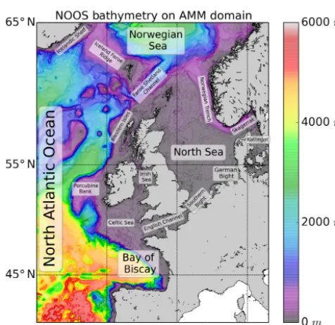
The European north-west shelf (NWS) is an area of intense socioeconomic interest with a wide variety of dynamical regimes. It is a region that has been the subject of numer-ous research models over many years both domain-wide and focusing on smaller subregions. Research models and as-sociated assimilation schemes for the region have matured into a number of operational systems. As part of the Coper-nicus Marine Environment Monitoring Service (CMEMS), an operational forecast system based on the Atlantic Margin Model (AMM) domain (O’Dea et al., 2012) has been devel-oped to provide products for coastal modelling downstream users. The AMM term refers to the model domain rather than the full configuration for the NWS as implemented at the Met Office. It is the model domain of previous Met Office NWS configurations up to and including CO5, and it is shown in Fig. 1.
Figure 1.NOOS bathymetry for the AMM domain.
past decades but also provide a way to assess and validate the operational systems over longer periods against historical data. The presentation of systematic biases and drifts allows the users to understand the limitations and appropriateness of a particular product to their interest or application. Fur-thermore, as systems are upgraded, the associated reanalyses provide a means to intercompare and evaluate the effective-ness of system updates.
Here, we describe the non-assimilating standard Coastal Ocean configuration version 5 (CO5) control hindcast. This CO5 hindcast provides a reference to understand underly-ing biases and drifts attributable to changes in the physics updates alone. CO5 includes all input parameters, ancillary files, model code and compilation keys required to run the model. CO5 forms the physics component of the Coperni-cus reanalysis product replacing the preexisting POLCOMS-derived hindcast product. In support of the full reanalysis, a non-assimilative control hindcast was integrated from Jan-uary 1981 to June 2012. CO5 was jointly developed by the Met Office and the National Oceanography Centre. Standard configurations such as CO5 are subsequently incorporated as constituent parts of broader modelling systems such as cli-mate projections (Tinker et al., 2015) or coupled systems (Sikiri´c et al., 2013).
CO5 is an update of the Nucleus for European Modelling of the Ocean (NEMO) (Madec, 2008) configuration used to model the NWS in O’Dea et al. (2012). For convenience, we reference the configuration in O’Dea et al. (2012) as CO4. CO4 was also based on the operational AMM domain at the Met Office. Changes include new riverine forcing, updated Baltic boundary conditions, increased vertical resolution, dif-ferent surface forcing, as well as an updated base NEMO
from version 3.2 to 3.4. The CO5 reanalysis product is an update to the 12 km POLCOMS hindcast (Holt et al., 2012) for 1965–2004 of the same AMM region. We compare the CO5 non-assimilative control hindcast with the POLCOMS hindcast over common years of integration for the period 1985–2004 and exclude the CO5 spin-up years 1981–1984. Both are compared against standard climatologies and obser-vations. Individual updates incorporated into CO5 are also investigated systematically by a series of 30-year sensitivity experiments, looking at the changes in isolation. The surface and boundary forcing datasets used in CO4 only start from 2006, so it is not possible to do a full 30-year like-for-like CO4 and CO5 comparison. However, shorter 5-year experi-ments looking at the effects of the forcing are also investi-gated.
The structure of the paper is as follows. Section 2 gives an overview of the standard configuration CO5. Configura-tion updates are detailed in Sect. 3. The experimental design including the specifics of the sensitivity experiments are out-lined in Sect. 4. Section 5 has three main subsections:
– Section 5.1 is concerned with tidal analysis of CO5. – Section 5.2 isolates long-term biases compared to
cli-matology, observations and the POLCOMS hindcast. – Section 5.3 presents results from sensitivity experiments
that look in isolation at changes brought into CO5. Section 6 summarises and discusses the results before com-menting on future system upgrades which are informed by the analysis of this paper.
2 Core model description
CO5 builds upon and thus shares many of the core features of the previous Met Office shelf seas model configuration CO4, as described in O’Dea et al. (2012). Elaboration of the key features particular to CO5 that are distinct from CO4 is deferred to Sect. 3.
(200 km), it is not sufficient to resolve the internal Rossby ra-dius on the shelf which is of the order 4 km (Holt and Proctor, 2008). However, at the time of integration of the reanalysis, it was not computationally feasible to conduct multiple 30-year hindcasts of the CO5 domain with a resolution approaching the 1.5 km required to resolve the internal radius.
As tides and surges play such important roles on the Eu-ropean NWS, a non-linear free surface is implemented us-ing the variable volume layer (Levier et al., 2007) and time-splitting approaches in NEMO. The baroclinic time step used in the 30-year hindcasts of CO5 is 300 s with a barotropic time step of 10 s. The advection of momentum is both en-ergy and enstrophy conserving (Arakawa and Lamb, 1981). Both bi-Laplacian and Laplacian horizontal viscosities are applied. The Laplacian viscosity is applied along geopoten-tial levels with a coefficient of 30.0 m2s−1. The bi-Laplacian viscosity is used to retain model stability and is applied on model levels with a coefficient of 1.0×10⁻¹⁰m4s−1. The
lateral momentum boundary condition is free slip. Tracer ad-vection is implemented using the total variation diminish-ing (TVD) scheme (Zalesak, 1979). Unlike CO4, Laplacian tracer diffusion operates only along geopotential levels with a coefficient of 50 m2s−1.
The generic length scale (GLS) turbulence scheme calcu-lates the turbulent viscosities and diffusivities (Umlauf and Burchard, 2003). The second-moment algebraic closure of Canuto et al. (2001) is solved with two dynamical equations (Rodi, 1987) for the turbulence kinetic energy (TKE),kand TKE dissipation,(Umlauf and Burchard, 2005). At the sur-face and bed, Neumann boundary conditions onkandare applied. Surface wave mixing is parameterised as in Craig and Banner (1994). Dissipation under stable stratification is limited using the Galperin limit (Galperin et al., 1988) of 0.267. A spatially varying log-layer-derived drag coefficient with a minimum set at 0.0025 controls the bottom friction.
3 Summary of main model updates
CO5 has four configuration updates from CO4. These up-dates involve the vertical levels, the source riverine input, the treatment of the exchange with the Baltic through the Kat-tegat and the base version of NEMO. Furthermore, the in-puts at the oceanic lateral boundary conditions and the sur-face boundary condition (SBC) for the 30-year hindcast are substantially different from the shorter runs detailed for the forecast implementation of CO4 in O’Dea et al. (2012). Here, we describe in detail each of the changes, and in Sect. 4 a set of sensitivity experiments explores the impacts of these changes.
3.1 Vertical coordinate
The vertical coordinate in CO5 is inherited from CO4 and is az∗−σ coordinate. It is terrain following and is fitted to a
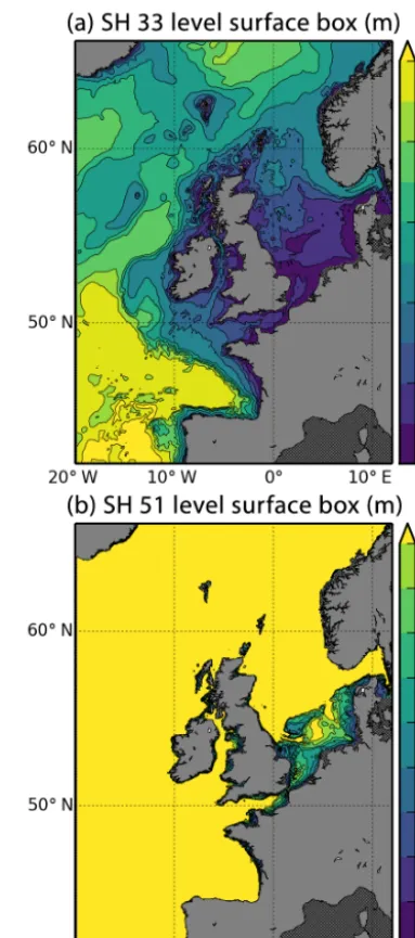
Figure 2. Thickness of surface model levels in CO4 (a) and CO5(b).
A comparison of the thickness of the surface model level in CO4 and CO5 is shown in Fig. 2. It is only in the shallow-est regions (bathymetry of less than 50 m) where the surface level thickness in CO5 is not set equal to 1 m, whereas in CO4 the surface model level varies considerably over the do-main from deep water to shelf. Thus, any change in CO5 that impacts upon air–sea exchange will be applied equally across most of the domain allowing cause and effect to be more readily parsed. Furthermore, follow-on configurations of CO5 will feature ocean–atmosphere coupling where again consistent air–sea exchange will be important.
3.2 Riverine input
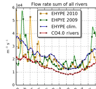
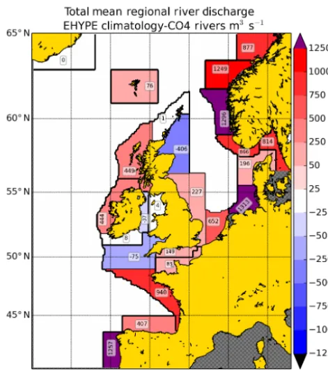
The second significant change between CO4 and CO5 is the data source for riverine input. In CO4, an annual cli-matology of some 320 European rivers mapped to 165 out-flow points on the CO4 grid constitutes the riverine in-put regardless of the model year (Young and Holt, 2007). As a step towards temporal variation and higher resolution of riverine sources, the old climatology is replaced with data from a pan-European implementation of the hydrolog-ical model HYdrologhydrolog-ical Predictions for the Environment (HYPE) (Lindström et al., 2010). The European implemen-tation of HYPE is known as E-HYPE (Donnelly et al., 2015) and has a sub-basin resolution of 120 km2. There is both an operational forecast and hindcast of E-HYPE, and the data are freely available at http://hypeweb.smhi.se/europehype/ long-term-means. Daily river outflow data are mapped to 476 outflow points on the CO5 grid from version 2.1 of E-HYPE. Data were provided by the Swedish Meteorological and Hy-drological Institute (SMHI) for the entire period of the hind-cast. The E-HYPE data provide a greater number of river sources along the coastline of continental Europe. Figure 3 compares the total riverine input from all rivers in the do-main for both the CO4 river climatology and the 1980–2012 mean of the E-HYPE data. Two individual years of E-HYPE data are also included to show the day-to-day and year-to-year variability that E-HYPE daily data contain compared to the climatological means. The difference in subregions along subsections of coast is shown in Fig. 4. The increase in con-tinental river outflow leads to the mean E-HYPE outflow be-ing considerably larger than the CO4 river climatology. How-ever, as presented in Fig. 4, the increase is not uniform and indeed the mean outflow from regions of the UK is actually slightly reduced in E-HYPE. In some areas, such as the Ger-man Bight and the Norwegian coast, E-HYPE outflow is sub-stantially increased.
3.3 Baltic exchange
The third update to CO5 concerns the exchange between the North Sea and the Baltic through the Danish straits and the Kattegat. At 7 km resolution, it is not possible to resolve the Danish straits, given that Öresund is 4 km wide at its
narrow-Figure 3.Comparison of total river flow rate between E-HYPE in-dividual years, 30-year mean and CO4 climatological rivers.
Figure 4.Comparison of coastal subsections of total river flow rate between E-HYPE and CO4 climatological rivers.
3.4 Surface boundary condition
The surface boundary condition in CO5 has also changed from CO4. In CO4, the surface boundary conditions are directly prescribed fluxes from the Met Office’s numerical weather prediction (NWP) model. Directly prescribed fluxes are replaced by calculating momentum, heat and freshwater fluxes using the Common Ocean-ice Reference Experiment (CORE) bulk formulae (Large and Yeager, 2009). The NWP data are only available from November 2006, and so a dif-ferent surface boundary condition must be used for the 30-year CO5 hindcasts starting in 1981. The atmospheric forc-ing dataset used to force the 30-year hindcast is the ERA-Interim dataset of the European Centre for Medium-Range Weather Forecasts (ECMWF) (Dee et al., 2011). In addition to switching to bulk formulae, the light attenuation scheme used in CO5 is also changed to the standard NEMO tri-band red–blue–green (RGB) scheme of Lengaigne et al. (2007). The RGB scheme replaces the single-band scheme presented in Holt and James (2001) which is used in CO4. We refer to this single-band scheme as PDWL in this paper. One conse-quence of this change in the light scheme in CO5 is that the extinction depths do not vary across the domain in propor-tion to the bathymetry as in CO4 and POLCOMS. The vari-ance in extinction depth was a first-order attempt to mimic the change in water clarity from deep waters to shallow.
4 Experimental design
The CO5 control run forms the baseline experiment for this paper. This baseline control run and the older POL-COMS hindcast are compared to evaluate how the two mod-elling systems perform irrespective of assimilation. The rele-vant configuration differences between CO5, CO4 and POL-COMS are shown in Table 1.
The configurations are compared with respect to satellite-derived sea surface temperature (SST), in situ subsurface ob-servations, as well as both global and regional climatologies. To establish the effect of the key changes from CO4 to CO5, a set of sensitivity experiments are integrated over the full 30-year period. The key differences of the 30-30-year experiments are listed in Table 2.
The shorter CO4 experiments in O’Dea et al. (2012) used direct fluxes from NWP atmospheric forcing at v3.2 of NEMO. The Met Office NWP forcing dataset only covers November 2006–2012. Thus, to investigate the effect of the different surface forcing, a second set of experiments was in-tegrated. The key differences are shown in Table 3.
This second set of experiments also determines the dif-ference between upgrading the NEMO code and keeping all other parameters as similar as is feasible. In the CO4 ex-periments, there was also a bug involving the application of the inverse barometer at the lateral boundaries, and its effect is explored in the 5-year experiments by re-inclusion in one v3.4 experiment.
4.1 Model initialisation and forcing
CO5 was initialised in January 1981 by interpolating temper-ature and salinity fields from the 1/4◦ ORCA025 hindcast
Table 1.Key configuration differences.
Configuration POLCOMS CO4 CO5
Code base POLCOMS NEMO 3.4 NEMO3.6
Horizontal resolution 12 km 7 km 7 km
Vertical levels 40 SH levels 33 SH levels 51 SF levels
Surface forcing ERA40 NWP ERAI
Lateral boundary 1◦global North Atlantic 12 km 1/4◦global GO5.0 and GLOSEA5
River source Climatology Climatology E-HYPE
Baltic boundary Climatology at two points Climatology at two points IoW boundary condition
Light penetration PDWL PDWL RGB
Integration period 1960–2004 2007–2012 1981–2012
NWP refers to Met Office numerical weather prediction (NWP) fluxes directly prescribed. IoW refers to data from the IoW NSBS GETM model of the Baltic (Gräwe et al., 2015). RGB is the default tri-band light attenuation scheme in NEMO (Lengaigne et al., 2007). PDWL refers to the single-band scheme that varies attenuation in proportion to sea bed depth (Holt and James, 2001).
Table 2.The 30-year sensitivity experiments.
EXP Levels River Baltic Light
CNTL SF51 E-HYPE IoW RGB
S30_1 SH33 E-HYPE IoW RGB
S30_2 SH33 Climatology Climatology RGB
S30_3 SH33 Climatology IoW RGB
S30_4 SH33 E-HYPE Climatology RGB
S30_5 SF51 E-HYPE IoW PDWL
CNTL is the CO5 control. SF51 refers to 51 SF levels. SH33 refers to 33 SH levels. IoW refers to data from the IoW NSBS GETM model of the Baltic (Gräwe et al., 2015). RGB is the default tri-band light attenuation scheme in NEMO (Lengaigne et al., 2007). PDWL refers to the single-band scheme that varies attenuation in proportion to sea bed depth (Holt and James, 2001).
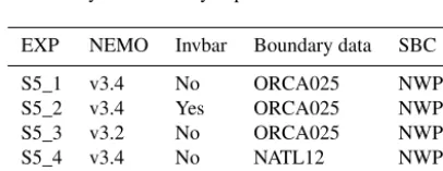
Table 3.The 5-year sensitivity experiments.
EXP NEMO Invbar Boundary data SBC
S5_1 v3.4 No ORCA025 NWP
S5_2 v3.4 Yes ORCA025 NWP
S5_3 v3.2 No ORCA025 NWP
S5_4 v3.4 No NATL12 NWP
S5_5 v3.4 No ORCA025 ERAI
All 5-year experiments use the single-band light attenuation of Holt and James (2001). S5_1–S5_4 use directly specified fluxes from the Met Office NWP model. S5_5 uses ERA-Interim (ERAI) derived fluxes as in the CO5 control. Versions v3.2 and v3.4 refer to the base version of NEMO. Invbar specifies whether the inverse barometer effect is added at the boundary or not. ORCA025 and NATL12 refer to the source model data used for the open lateral boundary conditions.
at 1 nautical mile resolution were made available from IoW for the years 2000–2012. For years prior to this, an annual cli-matology was created based on the 2000–2012 NSBS GETM data. In the control run, river forcings from E-HYPE data are utilised for the full 30-year hindcast. The sensitivity exper-iments include hindcasts with the climatological rivers and climatological Baltic boundary to understand the impacts of the newer inputs.
Table 4.Elevation RMSE of amplitude in centimetres as compared to observations.
M2 S2 K1 O1 N2
CO4 10.3 3.7 1.8 1.9 2.9
CO5 11.4 4.5 2.0 1.9 3.4
CO5* 9.5 4.0 1.8 1.6 3.3
CO5* refers to CO5 with lower reference density and time-splitting bug fix.
5 Results
5.1 Tidal harmonics
The co-tidal charts of the M2 SSH tidal harmonic, as anal-ysed from CO4 and CO5, are given in Fig. 5. Overall, the general representation is fairly similar. CO4 and CO5 broadly agree with amphidrome positions derived from ob-servations such as in Howarth and Pugh (1983). Whilst the position of degenerate amphidrome in southern Norway in CO5 may appear to align more closely with the observations, it must be noted that the data sparsity in this region is sig-nificant, and thus there is large uncertainty in the location of the degenerate amphidrome. In any case, it is found that the change in the land–sea mask from CO4 to CO5 due to the new Baltic boundary condition is the main driver behind the shift in the amphidrome rather than a targeted model im-provement for the amphidrome’s position. Two almost iden-tical integrations of CO5 with and without the Baltic bound-ary masking were integrated. In the integration with the CO4 mask, the amphidrome returns to the position calculated in CO4.
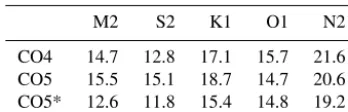
Table 5.Elevation RMSE of phase in degrees as compared to ob-servations.
M2 S2 K1 O1 N2
CO4 14.7 12.8 17.1 15.7 21.6 CO5 15.5 15.1 18.7 14.7 20.6 CO5* 12.6 11.8 15.4 14.8 19.2
CO5* refers to CO5 with lower reference density and time-splitting bug fix.
The CO5 configuration, as used in all sensitivity experi-ments in this paper, has a slightly larger RMSE in both am-plitude and phase compared to CO4. Two issues behind this increase in error were found. One was due to an order of cal-culation bug in the time splitting in CO5. This resulted in a small error in the surface pressure gradient term. The second was in relation to the reference density within NEMO. In the CO4 configuration, the reference density was 1027 kg m−3. However, in CO5, the NEMO v3.4 default of 1035 kg m−3 was used. When these were corrected for, CO5 slightly im-proves upon CO4 when compared to the standard observa-tions. To understand if these changes have any significant impact on the control and reanalysis, a further experiment with the changes was integrated. No significant difference in mean temperature or salinity fields was found.
5.2 Surface biases 5.2.1 Seasonal SST biases
The mean seasonal model SST from 1985 to 2004 is com-pared with remotely sensed products. These include the Na-tional Oceanic and Atmospheric Administration (NOAA) Advanced Very High Resolution Radiometer (AVHRR) product (Casey et al., 2010) and the European Space Agency (ESA) Climate Change Initiative (CCI) product (Merchant et al., 2014). The period 1985–2004 is chosen for two rea-sons. First, it allows for the CO5 hindcast to be spun up from rest in 1981. Secondly, it presents a common period with which to compare the POLCOMS hindcast that ends in 2005. Figure 6 compares the CO5 control and POLCOMS hind-cast SST bias against the AVHRR data. The largest bias in CO5 SST is the cold bias extending from eastern Iceland south-eastwards to the Faroe–Shetland Channel (FSC) and from the FSC north-westwards to the northern boundary of the domain. This SST bias is less apparent in summer as seen in Fig. 6c. The reduction in the bias might be caused by over-stratification in summer. The regions immediately surround-ing the cold bias area appear to be warm biased in summer. This suggests the cold bias may be of a remote origin such as the boundary condition. Elsewhere off shelf there is a smaller cold bias in winter, spring and autumn. Along the Celtic shelf break, there is a slight warm bias. The model is probably un-derestimating the cold water surface signal associated with
enhanced vertical mixing at the shelf break. In summer, off shelf southward of 50◦N, CO5 appears to be too warm. On
shelf, CO5 SST is slightly cold biased in most regions for most seasons.
However, there are some warm biases, particularly in sum-mer. The Southern Bight, the Western Isles of Scotland and the western Irish Sea all have summertime warm biases. The English Channel also has a warm SST bias in autumn.
Figure 6e–h show the equivalent seasonal SST bias for the POLCOMS hindcast. POLCOMS also has a large cold bias from Iceland to the FSC and from the FSC to the north-ern boundary in winter, spring and to some extent in au-tumn. However, the POLCOMS SST cold bias appears to be more extensive. It also extends south-westwards from the FSC to roughly the Porcupine Bank. Near the western bound-ary, there is also a significant warm SST bias in POLCOMS north of 55◦N in winter. Off shelf in summer, there is a large
warm bias in POLCOMS across much of the domain. How-ever, there is also a large summertime SST cold bias in the Norwegian Trench, the Skagerrak and the Kattegat.
In summary, the CO5 control hindcast appears to have a much smaller SST bias than the preceding POLCOMS hind-cast. One particularly large bias in CO5 is the large cold bias in the northern part of the domain which is also present in POLCOMS. This bias is explored further with comparisons against temperature and salinity profiles, as well as climatol-ogy. CO5 does appear to be too warm off shelf in summer but much less so than POLCOMS. On shelf, CO5 is generally slightly cold biased, whereas POLCOMS alternates from a large wintertime cold bias to a large summertime warm bias. POLCOMS is too cold in the Norwegian Trench during sum-mer, while CO5 appears to do reasonably well there.
5.2.2 Surface salinity biases
The mean sea surface salinity (SSS) of CO5 for 1985–2004 and the POLCOMS hindcast are compared against the World Ocean Atlas 2013 (WOA13) global climatology (Zweng et al., 2013), the KLIWAS North Sea climatology (KLIWAS) (Bersch et al., 2013) and EN4 (Good et al., 2013) profile data in Fig. 7. A similar pattern in negative SSS bias as SST bias from Iceland to the FSC and to the northern boundary is present in CO5. With the exception of this northern re-gion, CO5 off shelf is in reasonably good agreement with both the climatology and the mean profiles. However, POL-COMS appears too fresh off shelf except along the western French coast, indicating an offset in surface salinity between CO5 and POLCOMS. On the shelf, CO5 is in general slightly too saline. In particular, the Irish Sea is saline biased in CO5 and indicates the E-HYPE freshwater flux may be too small there.
Norwe-Figure 5.M2 co-tidal charts.(a)CO4, NEMO v3.2.(b)CO5, NEMO v3.4.
Figure 6.The difference between the mean seasonal model SST and the mean satellite SST for 1985–2004.(a)CO5 December–January– February (DJF) bias,(b)CO5 spring March–April–May (MAM) bias,(c)CO5 summer June–July–August (JJA) bias,(d)CO5 autumn bias September–October–November (SON),(e)POLCOMS (POLC) winter (DJF) bias,(f)POLC spring (MAM) bias,(g)POLC summer (JJA) bias and(h)POLC autumn bias (SON).
gian coast it is too fresh and near the western limb of the Norwegian Trench it is too saline. In POLCOMS, not only are there fewer vertical levels but the vertical resolution near the surface is proportional to the ocean depth as in CO4. Con-sequently, compared to CO5, the surface resolution in
Figure 7.Mean model sea surface salinity (SSS) differences 1985–2004 from WOA13, KLIWAS and EN4:(a)CO5 – WOA13 climatology, (b)POLCOMS – WOA13 climatology,(c)O5 – EN4,(d)POLCOMS – EN4,(e)CO5 – KLIWAS North Sea climatology,(f)POLCOMS – KLIWAS North Sea climatology,(g)CO5 – EN4 in the North Sea and(h)POLCOMS – EN4 in the North Sea.
also more similar to CO4 than CO5 when using climatolog-ical river points to represent the exchange with the Baltic. The sensitivity experiments below investigate the effect of both these changes within the NEMO framework. With re-gards to the dipole in CO5, the resolution at 7 km is not suf-ficient to resolve the intense mixing processes in the trench where northward-flowing freshwater of Baltic origin along the Norwegian coast mixes laterally with adjacent incoming southward-flowing saline Atlantic water. It is anticipated that with increased horizontal resolution, better representation of eddy-induced mixing may reduce the dipole there.
POLCOMS and CO5 have biases of opposite signs in the German Bight; CO5 is too fresh and POLCOMS is too saline. POLCOMS uses the climatological rivers as in CO4 in con-trast to the E-HYPE rivers used in CO5. Thus, the sensitivity experiments S30_1, S30_2 and S30_3 that compare the dif-ferent river sources should help to understand the difference in this bias. POLCOMS also appears to be too fresh in the Southern Bight, and this may be contributing to the saline bias in the German Bight. POLCOMS may not be advecting the Rhine outflow to the east close enough to the coast. CO5 in contrast appears to be too fresh in the vicinity of the Rhine outflow.
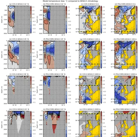
5.2.3 Off-shelf temperature and salinity biases through depth against WOA13 climatology
To assess how CO5 and POLCOMS behave throughout the water column off shelf, they are compared against WOA13 data. Figure 8 displays both zonal transects and depth level temperature biases for 1985–2004 compared to WOA13. Both CO5 and POLCOMS temperature biases are included in Fig. 8. Figure 9 is the equivalent salinity plot. As the mean is for the entire period, seasonal biases such as in the SST plots of Fig. 6 are not discernible. The location of the transects are chosen to intersect regions of particularly large bias. Note that these comparisons use the CMEMS POLCOMS dataset, which was interpolated onto standard depth levels from the native POLCOMS grid which uses 40 s levels in the verti-cal (Holt et al., 2012). The interpolated POLCOMS data are particularly coarse at depth which is reflected in the step-like nature of the POLCOMS bias plots at depth. This accounts for some of the differences seen towards the bottom of pro-files in Fig. 8.
orig-Figure 8.CO5 and POLCOMS temperature bias compared to WOA13 1985–2005. Panels(a),(e),(i)and(m)are CO5 – WOA13 temperature bias transects along 42, 45, 58 and 63◦N. Panels(b),(f),(j)and(n)are POLCOMS – WOA13 temperature bias transects along 42, 45, 58 and 63◦N. Panels(c),(g),(k)and(o)are the CO5 – WOA13 temperature bias at depths 0, 100, 1000 and 2000 m. Panels(d),(h),(l)and(p) are the POLCOMS – WOA13 temperature bias at depths 0, 100, 1000 and 2000 m.
inates near the southern boundary away from the relaxation zone. A warm temperature bias surrounds the cold temper-ature bias away from the coast. A similar pattern in salinity bias is shown in Fig. 9. It appears the models are diffusing both horizontally and vertically the warm and saline waters of Mediterranean origin entering the domain from the south-ern boundary. The extra diffusion in the relaxation zone and the relatively coarse vertical resolution of about 100 m at a depth of 1000 m may be contributing to the loss in identity of
the Mediterranean waters. The anomaly is also present in the Bay of Biscay but is much reduced in CO5 further north.
POL-COMS is quite coarse at this depth. However, it suggests that at depths greater than 500 m POLCOMS is warm biased in the FSC and Norwegian Sea, and CO5 appears to be close to the climatology below 500 m. There is a similar pattern in the salinity bias with both CO5 and POLCOMS relatively fresh near the surface in this region. On the other hand, POL-COMS appears to be slightly fresher than WOA13 off shelf right through depth for most of the domain. Off shelf, away from Biscay and the northern boundary, CO5 salinity is quite similar to WOA13.
5.2.4 North Sea temperature and salinity biases through depth
The KLIWAS climatology for the NWS in combination with EN4 provides an alternative to WOA13 for evaluation of the models on the shelf itself. Figures 10 and 11 compare CO5 with both the KLIWAS climatology and the EN4 data over the period 1985–2004. A comparison of POLCOMS against KLIWAS is also included as a reference. Figure 10 focuses on the summer months when there is seasonal thermal strat-ification, while Fig. 11 is the salinity mean for all seasons. Including all seasons allows for a larger number of in situ profiles to compare against. In addition to biases at depth lev-els of 10, 30 and 40 m, transects are taken through areas of significant bias to give an overview of the vertical structure in the model bias.
Generally, the structure of the temperature bias between CO5 and EN4 is in reasonable agreement with the structure of the bias between CO5 and the KLIWAS climatology. In the seasonally stratified areas of the North Sea, CO5 com-pares favourably near the surface compared to POLCOMS. POLCOMS there is significantly warm biased. Immediately below the thermocline, both CO5 and POLCOMS are cold biased with the cold bias in POLCOMS being somewhat larger than CO5. In CO5, the cold bias does not extend to the bed and in fact reverses sign to be warm biased near the bed, whilst in POLCOMS the cold bias reduces towards the bed with only a small bias remaining at the sea floor. The light attenuation schemes in CO5 and POLCOMS are quite different and may partially explain why POLCOMS is more warm biased at the surface and more cold biased at depth. The light scheme used in POLCOMS (PDWL) is also imple-mented in CO4 and is included in the sensitivity experiments to enable its impact to be assessed.
The CO5 salinity bias against EN4 is also broadly in agree-ment with the bias against the KLIWAS climatology. As in the surface plots of Fig. 7, over most of the North Sea, CO5 is slightly too saline through depth. Along the coasts of Hol-land, Germany and Denmark, CO5 is clearly too fresh, sug-gesting too much riverine input as discussed earlier. Away from the coasts, POLCOMS is in fairly good agreement with EN4 and KLIWAS while just slightly fresher at depth. The transects in Fig. 11 are taken to go through the Norwegian Trench and the Rhine plume. CO5 is shown to be roughly 0.5
too fresh above 20 m in the Norwegian Trench near the coast of Norway, while below 20 m CO5 is slightly too saline. The warmer and more saline water from the Atlantic appears to make CO5 too saline along the rim of the Norwegian Trench. In contrast, POLCOMS is shown to be typically greater than 1.1 too saline above 20 m in the Norwegian Trench, while be-low 40 m, POLCOMS switches from the large saline bias to a significantly fresh bias. It appears that CO5 is representing the haline stratification in the Norwegian Trench with greater fidelity than POLCOMS. Both the vertical resolution and the Baltic boundary condition may play some role in this and are included in the sensitivity experiments that follow.
5.3 The 30-year sensitivity runs
5.3.1 Vertical levels and stretching function
The effect of the changes of surface vertical resolution be-tween CO4 and CO5 is shown in Fig. 2. Sensitivity experi-ment S30_1 is exactly the same as the control (CNTL) ex-cept it uses 33 SH vertical levels instead of 51 SF levels. Although there are some small changes in summertime strat-ification off the shelf, the most dramatic change concerns the surface salinity in the Norwegian Trench. Figure 12 is the difference in salinity at 5 m between the control experiment CNTL (SF51) and sensitivity experiment S30_1 (SH33). The extra vertical resolution in the control run results in less dif-fusion of the surface fresh layer with depth. The POLCOMS hindcast also has much less vertical resolution at the surface than CO5, which may be one factor underlying its saline bias in the surface waters of the Norwegian Trench.
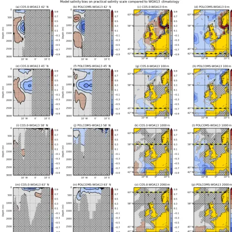
5.3.2 Baltic and rivers
Figure 9.CO5 and POLCOMS salinity bias compared to WOA13 for 1985–2005. Panels(a),(e),(i)and(m)are CO5 – WOA13 salinity bias transects along 42, 45, 58 and 63◦N. Panels(b),(f),(j)and(n)are POLCOMS – WOA13 salinity bias transects along 42, 45, 58 and 63◦N. Panels(c),(g),(k)and(o)are the CO5 – WOA13 salinity bias at depths 0, 100, 1000 and 2000 m. Panels(d),(h),(l)and(p)are the POLCOMS – WOA13 salinity bias at depths 0, 100, 1000 and 2000 m.
the mean transport across selected NOOS transects into and out of the North Sea. The calculated transports are similar to reported values from observational estimates as shown in Table 6.
Around parts of the coast of the UK, the E-HYPE river discharge in some regions is actually slightly less than the climatology or only slightly greater in others. This is also re-flected in the difference of salinity shown in Fig. 13c. Com-bining the correlation between areas of larger E-HYPE river
discharge than climatological rivers and the larger salinity biases in CO5 with what appears reasonable transports in CO5, it seems likely that the E-HYPE rivers are the first-order source of the salinity biases observed in CO5.
Figure 10.North Sea temperature bias compared to EN4 and the KLIWAS climatology for summer (JJA). Panels(a)–(d)compare CO5 and EN4 at 10, 30 and 40 m and along a transect at 56◦N. Panels(e)–(h)compare CO5 and KLIWAS climatology at 10, 30 and 40 m and along a transect at 56◦N. Panels(e)–(h)compare POLCOMS and KLIWAS climatology at 10, 30 and 40 m and along a transect at 56◦N. Panels(m)–(o)are transects through depth for each case along longitude 2.8◦E.
Table 6.Net transports across NOOS sections.
Name NOOS ID Paper reference Observational value CO5 value
Feie–Shetland west 1 Otto et al. (1990) 0.6 Sv 0.54 Sv
Feie–Shetland east 2 Otto et al. (1990) 0.7–1.1 Sv 1.11 Sv
Orkney–Shetland 3 Otto et al. (1990) 0.3 Sv 0.4 Sv
Figure 11.North Sea salinity bias compared to annual EN4 and KLIWAS climatology. Panels(a)–(d)compare CO5 and EN4 at 6, 20 and 30 m and along a transect at 58◦N. Panels(e)–(h)compare CO5 and KLIWAS climatology at 6, 20 and 30 m and along a transect at 58◦N. Panels(e)–(h)compare POLCOMS and KLIWAS climatology at 6, 20 and 30 m and along a transect at 58◦N. Panels(m)–(o)are transects through depth for each case along longitude 4.8◦E.
to the E-HYPE rivers resulting in an overall freshening com-pared to the climatologies.
5.3.3 Light attenuation
The summertime biases in temperature were shown to be sig-nificantly different between POLCOMS and CO5. Sensitiv-ity experiment S30_5 explores replacing the light
dif-Figure 12.Comparison of mean salinity at 5 m between CO5 with 51 vertical levels using the Siddorn and Furner stretching func-tion (CNTL) and 33 vertical levels using the Song and Haidvogel stretching function (S30_1). The hashed area in the Kattegat indi-cates the interface to Baltic NSBS model data.
Figure 13.Comparing SSS using climatological river and Baltic in-puts against E-HYPE rivers and IoW Baltic. Panel(a)shows 33 SH levels with E-HYPE rivers and IoW Baltic (S30_1) vs. EN4. Panel (b)shows 33 SH levels with climatological rivers and climatolog-ical Baltic (S30_2) vs. EN4. Panel(c)shows climatological rivers minus E-HYPE rivers (S30_3–S30_1). Panel(d)shows climatolog-ical Baltic – IoW Baltic (S30_4–S30_1).
Figure 14.CO5 mean transport across selected NOOS transects sur-rounding the North Sea and the CO5 transport field shown only ev-ery fourth grid point for clarity.
ferently in each scheme and influences the degree of bias at the surface. In the PDWL scheme, all of the non-penetrating part is added to the surface layer, while in the RGB scheme there is still a slight penetration of the quickly attenuating light. The cold bias in both models indicates that the depth of the thermocline is too shallow, which could be either be due to the light not penetrating far enough in both schemes or insufficient vertical mixing. At depth, the PDWL scheme results in less heat being mixed down, resulting in a better agreement with the bed temperature as the RGB scheme is biased warm there. However, in mixed areas on shelf, both models appear to be too warm, which may indicate a bias in the surface flux forcing.
Figure 15b compares each scheme against the mean of the profiles off shelf south of 60◦N. Figure 15b does not show
Figure 15.Comparison of summertime profiles compared to NEMO’s three-band light attenuation scheme (RGB) and POLCOMS single-band scheme (PDWL). Panel(a)compares CNTL and S30_5 against the mean of profiles in the seasonally stratified part of the domain on shelf. Panel(b)compares CNTL and S30_5 against the mean of profiles off shelf south of 60◦N.
5.4 The 5-year sensitivity runs
The shorter CO4 experiments of O’Dea et al. (2012) used different open ocean boundary conditions and surface bound-ary conditions relative to the CO5 control run. To further ex-plore CO4 and CO5 differences whilst using the same forc-ing conditions of CO4, a set of sensitivity experiments for 5 years were undertaken starting in November 2006. The constraint on the start date is the availability of Met Office NWP flux data and the open boundary conditions used in CO4 which start from November 2006. All the 5-year ex-periments as detailed in Table 3 have 33 vertical levels with the Song and Haidvogel stretching function (Song and Haid-vogel, 1994). They also use climatological rivers, climato-logical Baltic and the single-band light attenuation scheme implemented in CO4. The sensitivity of the model to the vertical coordinate, rivers, the Baltic boundary and the light attenuation scheme is explored in the 30-year experiments in Sect. 5.3. They are not shown to have significant impact on the large SST bias from Iceland to the Faroe Islands. In the following sections, the effects of changed boundaries and fluxes with an emphasis on the sensitivity of the SST bias to these changes is detailed.
5.4.1 Inverse barometer and open ocean boundary condition
The 5-year sensitivity experiments show that the most sig-nificant differences between CO4 and CO5 are related to the lateral boundary conditions. A bug in NEMO v3.2 prevented
the application of the inverse barometer effect on the open ocean lateral boundaries. Thus, two sensitivity experiments with NEMO v3.4 were conducted: S5_1 with this bug de-liberately included and S5_2 without. An additional exper-iment, S5_3, is an equivalent experiment with exactly the same forcing but with NEMO v3.2 as the base model.
Figure 16.Isolating the difference in northern SST bias between CO4 and CO5. Panel(a)shows the mean SST difference between the NEMO v3.4 with the inverse barometer applied to the boundary and without (S5_2–S5_1). Panel(b)shows the mean SST difference between NEMO v3.4 with the inverse barometer applied to the boundary and NEMO v3.2 (S5_2–S5_3). Panel(c)shows the mean SST difference between NEMO v3.4 with ORCA025 and NATL12 boundary data (S5_4–S5_1). Panel(d)shows the difference between SST RMSE between NEMO v3.4 with the inverse barometer applied to the boundary and without (S5_2–S5_1). Panel(e)shows the difference between SST RMSE between the NEMO v3.4 with the inverse barometer applied to the boundary and NEMO v3.2 (S5_2–S5_3). Panel(f)shows the difference of SST RMSE between NEMO v3.4 with ORCA025 and NATL12 boundary data (S5_4–S5_1).
Another significant difference was the open ocean source data interpolated onto the open boundaries of CO5 and CO4. The 30-year sensitivity experiments of CO5 used data from the 1/4◦global ocean domain (ORCA025). However, CO4 was forced using a 1/12◦model of the North Atlantic (NATL12). In operational implementation of CO5, the higher resolution NATL12 model is also used to derive open bound-aries. Sensitivity experiment S5_4 is exactly the same as S5_1 but replaces the ORCA025-derived boundaries with boundaries derived from the NATL12 model. The mean and RMSE SST differences between S5_1 and S5_4 are shown in Fig. 16c and f. The NATL12 data result in a warmer SST from Iceland to the Faroe Islands and a reduced RMSE com-pared to the ORCA025 data.
The GLOSEA5 surface data are compared against WOA13 in Fig. 17. Compared to WOA13, GLOSEA5 is anomalously cold and fresh along the CO5 boundary of 65◦N. This suggests that a significant component of the northern bias in CO5 originates in the global model that pro-vides its northern boundary condition.
Figure 18.Comparison of mean SST(a)and SSS(b)differences between ERAI fluxes and NWP fluxes (S5_1 vs. S5_5).
5.4.2 Surface fluxes
Another important difference between CO4 and CO5 is the surface fluxes. In operational implementation, the surface fluxes are taken from the Met Office NWP model. The ex-periments in O’Dea et al. (2012) were also forced with NWP directly prescribed fluxes. However, comparable NWP model data were not available from before 2006, and thus the longer runs, as in the CO5 control, use ERAI surface fluxes. Further-more, the NWP fluxes are directly prescribed in contrast to the CORE bulk formulae used with ERAI. A Haney correc-tion (Haney, 1971) must also be applied when using direct fluxes with a prescribed reference SST as used by the NWP model itself.
Sensitivity experiment S5_5 is exactly as S5_1 but with ERAI-derived fluxes instead of NWP fluxes. Figure 18a and b compare the mean SST and SSS between S5_5 and S5_1. The SST is almost uniformly warmer with NWP fluxes than ERAI-derived fluxes, particularly in the Bay of Biscay, around the coast of the UK and into the Skagerrak and south-ern Norwegian Trench.
However, it should also be noted that because direct fluxes use the Haney correction, the resulting model SST is indi-rectly relaxed to the prescribed SST in a hindcast simula-tion. Furthermore, in NEMO version 3.2, the surface stress from direct fluxes was based on absolute wind velocity rather than wind velocity relative to the moving ocean surface. This has important localised effects in the vicinity of persistently strong surface currents, such as the Skagerrak. This sensi-tivity of the model to relative winds versus absolute winds using ERAI-derived forcing is also investigated. Figure 19 is the difference in the mean for 1 year of surface stress, salin-ity, current and temperature between using the relative wind velocity to the ocean surface and the absolute wind velocity. Furthermore, the details of the fluxes near coastlines, and particularly the wind stress in the Skagerrak and southern Norwegian Trench, are quite different between the lower-resolution ERAI and higher-lower-resolution NWP fluxes. The dif-fering resolution of the surface forcing and the use of
abso-Figure 19.Comparison between using wind velocity relative to ocean surface and absolute wind velocity for the 2011 annual mean. Panel(a)shows the difference in surface shear stress in Pa. Panel (b)shows the difference in surface salinity. Panel(c)shows the dif-ference in surface current. Panel(d)shows the difference in surface temperature.
lute instead of relative wind stress is thus likely to play a role in the different sensitivity experiments.
In Fig. 18b, it is shown that the experiment with ERAI-derived forcing is slightly more saline on shelf but signifi-cantly fresher in the Skagerrak and the Norwegian Trench mirroring the SST differences there. The difference in the shear stress modifies both the transport of the surface fresh layer out of the Skagerrak and the transport of relatively saline water from the North Sea into the Skagerrak. The difference in relative and absolute winds is significant also along the shelf break from the Shetland Islands northwards. In this case, the effect of using the absolute wind velocity is to reduce the transport of North Atlantic water northwards, which results in locally lower mean SST. With respect to the difference between ERAI-derived forcing and NWP-forced experiments, the difference in the SST in this local region is reduced. The reduction in the mean difference of SST is due to the countervailing effects of general domain-wide cold bias between ERAI-derived forcing and NWP fluxes, and the local cooling due to using absolute winds with the direct NWP fluxes.
6 Summary and discussion
model forms the basis of the physics component of the cur-rent CMEMS reanalysis of the NWS, which also includes data assimilation. CO5 is a regional tidal implementation of NEMO version 3.4, building upon CO4 (O’Dea et al., 2012) which used NEMO version 3.2 as the base code. In this paper, a 30-year physics-only control of CO5 using ERAI-derived surface forcing and ORCA025 lateral boundary conditions has been assessed against standard climatologies and obser-vations to understand the impact of model physics on biases. The assessment compares CO5 to a POLCOMS-based hind-cast over the period 1985–2004, which is a period covered by both hindcasts. A set of 30-year sensitivity hindcasts has also been assessed to understand several changes, relative to CO4, introduced into CO5. A further set of 5-year sensitivity ex-periments focusing on different surface and lateral boundary conditions has also been investigated.
Overall the CO5 tides are of comparable quality to CO4. The reference density of 1035 kg m−3 used in the control
run slightly degraded the tidal predictions. The position of the degenerate amphidrome in southern Norway is slightly changed in CO5 mainly due to a small modification the land– sea mask originating from a change in the Baltic boundary condition.
Compared to AVHRR data, CO5 has a large SST bias extending from Iceland to the FSC. It is particularly pro-nounced in winter and partially obscured in summer due to surface heating. POLCOMS also has a large seasonal cold SST bias in the region but also a significant warm SST bias domain-wide in summer. In comparison to the AVHRR ob-servations, CO5 appears to significantly improve upon the simulation of SST in the POLCOMS hindcast.
As in the SST, CO5 has a similar pattern of fresh bias in the near-surface salinity from Iceland to the FSC as well as a large fresh bias in the German Bight due to E-HYPE rivers and a dipole of surface salinity bias along the Norwegian Trench that suggests insufficient lateral mixing. POLCOMS, in contrast, is slightly too saline in the German Bight and uni-formly too saline at the surface along the Norwegian Trench. Both CO5 and POLCOMS appear to lose the identity of relatively warm saline Mediterranean water near the south-ern boundary of the domain. In CO5, there is a sponge layer in the boundary relaxation zone where the diffusion is in-creased for model stability. Furthermore, the vertical reso-lution is focused on the surface and bed and is particularly coarse mid-water in the deeper parts of the domain. Both of these may be contributing to the apparent overestimation of diffusion of this water mass both laterally and vertically.
In the North Sea, there is a marked difference in the ver-tical summer temperature profile between POLCOMS and CO5 in seasonally stratified regions. Compared to climatol-ogy and observations, POLCOMS is much too warm at the surface, while both POLCOMS and CO5 are too cold mid-water, and CO5 is too warm towards the bed.
The single-band light scheme (PDWL) used in POL-COMS and CO4 was seen to significantly alter the
temper-ature profile in seasonally stratified regions in CO5. Intro-ducing the PDWL scheme into CO5 leads to a larger warm bias at the surface and a larger colder mid-water cold bias than the CO5 control. From 40 m to the bed, the PDWL light attenuation scheme resulted in closer agreement with clima-tology than the CO5 control run. Both models appear to be over-stratifying with a very abrupt thermocline. Whilst the light attenuation scheme may be a component of this error, the vertical mixing will also be an important contributor and should be a subject of further refinement.
The sensitivity experiments also explored the significance of changing the riverine inputs and the Baltic boundary con-dition. The older climatological rivers greatly reduce the freshwater bias in the German Bight and also near the Nor-wegian coast. It appears that the version of E-HYPE used in CO5 has too much freshwater discharge from continental Eu-rope. The Baltic boundary condition used in CO5 results in slightly more saline surface waters in the Norwegian Trench. The added variability introduced by the CO5 Baltic bound-ary relative to the CO4 climatological boundbound-ary cannot be assessed by the long-term climatological means used in this paper. Further site-specific studies in the Kattegat and Sk-agerrak are required to evaluate the variability.
The impact of the change in vertical levels has a signifi-cant impact on the mean surface salinity in the Norwegian Trench. The increase in surface resolution allows retention of the relatively fresh layer of Baltic origin more than the coarser vertical levels used in CO4.
The 5-year sensitivity experiments revealed that a bug fix in CO5 related to the application of the inverse barometer ef-fect on the lateral boundaries results in a colder SST from Iceland to the FSC. This is the region where CO5 has a particularly large SST cold bias and partially explains why CO5 has larger SST errors here than CO4. The inclusion of the inverse barometer effect on the boundaries results in a greater transport of water southwards from the northern boundary and with it colder fresher water. The source data for the boundaries themselves also have a significant impact in this region. The higher resolution 1/12◦NATL12 model results in smaller cold bias there also. It is likely that 1/4◦ ORCA025 global model lacks sufficient resolution to model the Icelandic shelf in the vicinity of the northern CO5 bound-ary. The increased southwards transport of water from the northern boundary condition due to the inclusion of the in-verse barometer effect amplifies the cold and fresh anomaly of the ORCA025 boundary data.
rather than the relative wind velocity compared to the mov-ing ocean surface. The effect of usmov-ing relative versus absolute wind velocities has important impacts in localised regions with persistent strong surface currents such as the Skager-rak. The ERAI-derived forcing is also of a relatively coarse resolution and the details of near-coastal fluxes are quiet dif-ferent from the NWP fluxes. The combined difference of ab-solute versus relative winds and differing details in the fluxes combine to have significant impacts on surface transport and hence surface salinity in local regions such as the Skagerrak. In summary, CO5 has been shown to produce a signifi-cantly improved hindcast of the NWS compared to POL-COMS against climatologies and observations. However, there are a number of notable biases in CO5 that need ad-dressing in future configurations. Particular issues relate to freshwater inputs from rivers, surface boundary conditions as well as seasonal stratification in the North Sea.
The next standard configuration CO6 will be an incre-mental update for the physics based on some of the lessons learned from CO5. The relative stability of physics develop-ments between CO5 and CO6 allows for significant updates to both data assimilation and biology components for the NWS forecast system. Physics changes will include updating the base version of NEMO to 3.6, updating the light attenu-ation to use satellite-observed climatology of ocean colour instead of a domain-wide coefficient. The river inputs will be from an updated climatology with reduced biases com-pared to the E-HYPE rivers used in CO5. However, a step change in the physics will occur in CO7 when the resolution will be increased from 7 to 1.5 km. CO7 will be of a suffi-cient resolution to resolve the internal Rossby radius on the shelf. Possible improvements include capturing to first or-der the generation of internal tides at the shelf break, resolv-ing mesoscale eddies and consequently enhanced mixresolv-ing in the Norwegian Trench and greatly improving bathymetry and coastline to name but a few. Furthermore, CO7 is being de-veloped in anticipation of the longer-term goals of coupling to wave, atmosphere and land system models. The aspiration is to drive towards eventual operational coupled implemen-tation for which CO7 will form the basis of the ocean model component.
Code and data availability. The model code for NEMO v3.4 is freely available from the NEMO website (www.nemo-ocean.eu). After registration, the FORTRAN code is readily available using the open-source subversion software (http:/subervsion.apache.org). Additional modifications to the NEMO3.4 trunk are required for CO5.0 and are merged into the CO5 package branch. The CO5 package branch is freely available from the NEMO repository under branches/UKMO/CO5_package_branch.
The NEMO namelist used for CO5 is publicly available at https://doi.org/10.13140/RG.2.2.17410.89286 (O’Dea, 2016b).
Appendix A: FPP keys used in CO5
Table A1.FPP keys used with the CO5 control experiment.
key_tide Activate tidal potential forcing
key_dynspg_ts Free surface volume with time splitting key_ldfslp Rotation of lateral mixing tensor key_iomput Input output manager
key_vvl Variable volume layer key_shelf Diagnostic switch for output
key_zdfgls Generic length-scale turbulence scheme key_bdy Use open lateral boundaries
key_amm Dimensions for AMM domain key_levels=51 Number of vertical levels
Appendix B: Adjusting the lateral open ocean boundary conditions
The lateral open ocean boundary conditions are derived from three separate 1/4◦ORCA025 experiments. The years 1981 to 1989 are also taken from the GO5.0 1/4◦ORCA025 hind-cast (Megann et al., 2014). The boundary conditions from 1989 onwards are taken from the two separate Global Sea-sonal Forecast system version 5 (GLOSEA5) (MacLachlan et al., 2015) experiments spanning 1989–2003 and 2003– 2012.
Each of ORCA025 experiments had substantially differ-ent mean SSH. They needed to be matched at the cross-over dates as closely as possible to prevent large shocks. The free-running model GO5 experiment for the 1980s was shown to have a term unrealistic drift in the mean SSH. This long-term trend is removed from the data before deriving bound-ary conditions. Furthermore, the first GLOSEA run does not have altimeter assimilation until 1992 and likewise has an un-realistic drift removed from these initial years (1989–1992).
Once the data are detrended, a mean SSH is calculated area wide at the cross-over dates in 1989 and 2003. The second GLOSEA dataset is taken as the reference. The difference in the mean SSH in the earlier detrended GO5.0 experiment at the 1989 crossover data is then subtracted from the entire period (1981–1989). This, in effect, is a uniform shift in SSH so that at the cross-over date the discrepancy is as reduced as possible. Similarly, the difference in the mean between the first GLOSEA run and the second is used to match the two in 2003. However, even after this prepossessing, there is still some transient adjustment in SSH, particularly so at the 2003 cross-over.
Appendix C: Other inputs
Competing interests. The authors declare that they have no conflict of interest.
Acknowledgements. Funding support is gratefully acknowledged from the Ministry of Defence, the Public Weather Service, the European Community’s Seventh Framework Programme FP7/2007–2013 under grant agreement no. 283367 (MyOcean2) and from the Copernicus Marine Environment Monitoring Service. We acknowledge use of the MONSooN system, a collaborative facility supplied under the Joint Weather and Climate Research Programme, a strategic partnership between the Met Office and the Natural Environment Research Council. We also acknowledge the Centre for Environmental Data Analysis (CEDA) for the use of JASMIN (Lawrence et al., 2013) for post-processing the model data.
Edited by: Robert Marsh
Reviewed by: Bruce Hackett and Robinson Hordoir
References
Arakawa, A. and Lamb, V. R.: A potential enstrophy and en-ergy conserving scheme for the shallow water equations, Mon. Weather Rev., 109, 18–36, 1981.
Bersch, M., Gouretski, V., Sadikni, R., and Hinrichs, I.: KLIWAS North Sea Climatology of Hydrographic Data (Version 1.0), Tech. rep., Center for Earth System Re-search and Sustainability (CEN), University of Hamburg, https://doi.org/10.1594/WDCC/KNSC_hyd_v1.0, 2013. Canuto, V., Howard, A., Cheng, Y., and Dubovikov, M.: Ocean
tur-bulence. Part I: One-point closure model-momentum and heat vertical diffusivities, J/ Phys/ Oceanogr., 31, 1413–1426, 2001. Casey, K. S., Brandon, T. B., Cornillon, P., and Evans, R.:
The Past, Present, and Future of the AVHRR Pathfinder SST Program, Springer Netherlands, Dordrecht, 273–287, https://doi.org/10.1007/978-90-481-8681-5_16, 2010.
Craig, P. D. and Banner, M. L.: Modeling wave-enhanced turbu-lence in the ocean surface layer, J. Phys. Oceanogr., 24, 2546– 2559, 1994.
Dee, D., Uppala, S., Simmons, A. et al.: The ERA-Interim reanaly-sis: Configuration and performance of the data assimilation sys-tem, Q. J. Roy. Meteorol. Soc., 137, 553–597, 2011.
Donnelly, C., Andersson, J. C., and Arheimer, B.: Using flow signatures and catchment similarities to evaluate the E-HYPE multi-basin model across Europe, Hydrol. Sci. J., 61, 255–273, https://doi.org/10.1080/02626667.2015.1027710, 2015. Galperin, B., Kantha, L., Hassid, S., and Rosati, A.: A
quasi-equilibrium turbulent energy model for geophysical flows, J. At-mos. Sci., 45, 55–62, 1988.
Good, S. A., Martin, M. J., and Rayner, N. A.: EN4: Quality controlled ocean temperature and salinity pro-files and monthly objective analyses with uncertainty estimates, J. Geophys. Res.-Oceans, 118, 6704–6716, https://doi.org/10.1002/2013JC009067, 2013.
Gräwe, U., Holtermann, P., Klingbeil, K., and Burchard, H.: Advantages of vertically adaptive coordinates in numerical
models of stratified shelf seas, Ocean Model., 92, 56–68, https://doi.org/10.1016/j.ocemod.2015.05.008, 2015.
Haney, R. L.: Surface thermal boundary condition for ocean circu-lation models, J. Phys. Oceanogr., 1, 241–248, 1971.
Holt, J. and Proctor, R.: The seasonal circulation and vol-ume transport on the northwest European continental shelf: A fine-resolution model study, J. Geophys. Res.-Oceans, 113, https://doi.org/10.1029/2006JC004034, 2008.
Holt, J., Hughes, S., Hopkins, J., Wakelin, S. L., Holliday, N. P., Dye, S., González-Pola, C., Hjøllo, S. S., Mork, K. A., Nolan, G., Proctor, R., Read, J., Shammon, T., Sherwin, T., Smyth, T., Tattersall, G., Ward, B., and Wiltshire, K. H.: Multi-decadal vari-ability and trends in the temperature of the northwest European continental shelf: A model-data synthesis, Prog. Oceanogr., 106, 96–117, https://doi.org/10.1016/j.pocean.2012.08.001, 2012. Holt, J. T. and James, I. D.: An s coordinate density evolving model
of the northwest European continental shelf: 1. Model descrip-tion and density structure, J. Geophys. Res.-Oceans, 106, 14015– 14034, https://doi.org/10.1029/2000JC000304, 2001.
Howarth, M. and Pugh, D.: Chapter 4 Observations of Tides Over the Continental Shelf of North-West Europe, Elsevier Oceanog-raphy Series, 35, 135–188, https://doi.org/10.1016/S0422-9894(08)70502-6, 1983.
Ingleby, B. and Huddleston, M.: Quality control of ocean temperature and salinity profiles – Histori-cal and real-time data, J. Marine Syst., 65, 158–175, https://doi.org/10.1016/j.jmarsys.2005.11.019, 2007.
Large, W. and Yeager, S.: The global climatology of an interannu-ally varying air–sea flux data set, Clim. Dynam., 33, 341–364, 2009.
Lawrence, B. N., Bennett, V. L., Churchill, J., Juckes, M., Ker-shaw, P., Pascoe, S., Pepler, S., Pritchard, M., and Stephens, A.: Storing and manipulating environmental big data with JASMIN, in: 2013 IEEE International Conference on Big Data, 68–75, https://doi.org/10.1109/BigData.2013.6691556, 2013.
Lengaigne, M., Menkes, C., Aumont, O., Gorgues, T., Bopp, L., An-dré, J.-M., and Madec, G.: Influence of the oceanic biology on the tropical Pacific climate in a coupled general circulation model, Clim. Dynam., 28, 503–516, https://doi.org/10.1007/s00382-006-0200-2, 2007.
Levier, B., Tréguier, A. M., Madec, G., and Garnier, V.: Free surface and variable volume in the NEMO code, MESRSEA IP report WP09-CNRS-STR03-1A, 2007.
Lindström, G., Pers, C., Rosberg, J., Strömqvist, J., and Arheimer, B.: Development and testing of the HYPE (Hy-drological Predictions for the Environment) water quality model for different spatial scales, Hydrol. Res., 41, 295–319, https://doi.org/10.2166/nh.2010.007, 2010.
MacLachlan, C., Arribas, A., Peterson, K. A., Maidens, A., Fere-day, D., Scaife, A. A., Gordon, M., Vellinga, M., Williams, A., Comer, R. E., Camp, J., Xavier, P., and Madec, G.: Global Sea-sonal forecast system version 5 (GloSea5): a high-resolution sea-sonal forecast system, Q. J. Roy. Meteor. Soc., 141, 1072–1084, https://doi.org/10.1002/qj.2396, 2015.
Madec, G.: NEMO ocean engine: Note Du Pôle de Modél, Institut Pierre-Simon Laplace (IPSL), France, No 27, 2008.
coupled and forced applications, Geosci. Model Dev., 7, 1069– 1092, https://doi.org/10.5194/gmd-7-1069-2014, 2014.
Merchant, C. J., Embury, O., Roberts-Jones, J., Fiedler, E., Bulgin, C. E., Corlett, G. K., Good, S., McLaren, A., Rayner, N., Morak-Bozzo, S., and Donlon, C.: Sea surface temperature datasets for climate applications from Phase 1 of the European Space Agency Climate Change Initiative (SST CCI), Geoscience Data Journal, 1, 179–191, https://doi.org/10.1002/gdj3.20, 2014.
O’Dea, E.: CO5 Bathymetry,
https://doi.org/10.13140/RG.2.2.25799.50081, 2016a.
O’Dea, E.: CO5 AMM7 namelist,
https://doi.org/10.13140/RG.2.2.17410.89286, 2016b.
O’Dea, E. J., Arnold, A. K., Edwards, K. P., Furner, R., Hyder, P., Martin, M. J., Siddorn, J. R., Storkey, D., While, J., Holt, J. T., and Liu, H.: An operational ocean forecast system incorporating NEMO and SST data assimilation for the tidally driven European North-West shelf, Journal of Operational Oceanography, 5, 3–17, 2012.
Otto, L., Zimmerman, J., Furnes, G., Mork, M., Saetre, R., and Becker, G.: Review of the physical oceanogra-phy of the North Sea, Neth. J. Sea Res., 26, 161–238, https://doi.org/10.1016/0077-7579(90)90091-T, 1990.
Prandle, D., Ballard, G., Flatt, D., Harrison, A., Jones, S., Knight, P., Loch, S., McManus, J., Player, R., and Tappin, A.: Com-bining modelling and monitoring to determine fluxes of wa-ter, dissolved and particulate metals through the Dover Strait, Cont. Shelf Res., 16, 237–257, https://doi.org/10.1016/0278-4343(95)00009-P, 1996.
Rodi, W.: Examples of calculation methods for flow and mixing in stratified fluids, J. Geophys. Res.-Oceans, 92, 5305–5328, 1987. Siddorn, J. and Furner, R.: An analytical stretching function that combines the best attributes of geopotential and terrain-following vertical coordinates, Ocean Model., 66, 1–13, 2013.
Sikiri´c, M. D., Roland, A., Janekovi´c, I., Tomaz˘i´c, I., and Kuzmi´c, M.: Coupling of the Regional Ocean Modeling Sys-tem (ROMS) and Wind Wave Model, Ocean Model., 72, 59–73, https://doi.org/10.1016/j.ocemod.2013.08.002, 2013.
Song, Y. and Haidvogel, D.: A Semi-implicit Ocean Circu-lation Model Using a Generalized Topography-following Coordinate System, J. Comput. Phys., 115, 228–244, https://doi.org/10.1006/jcph.1994.1189, 1994.
Tinker, J., Lowe, J., Holt, J., Pardaens, A., and Wiltshire, A.: Valida-tion of an ensemble modelling system for climate projecValida-tions for the northwest European shelf seas, Prog. Oceanogr., 138, 211– 237, https://doi.org/10.1016/j.pocean.2015.07.002, 2015. Umlauf, L. and Burchard, H.: A generic length-scale equation for
geophysical turbulence models, J. Marine Res., 61, 235–265, 2003.
Umlauf, L. and Burchard, H.: Second-order turbulence closure models for geophysical boundary layers. A review of recent work, Cont. Shelf Res., 25, 795–827, 2005.
Young, E. and Holt, J.: Prediction and analysis of long-term vari-ability of temperature and salinity in the Irish Sea, J. Geophys. Res.-Oceans, 112, https://doi.org/10.1029/2005JC003386, 2007. Zalesak, S. T.: Fully multidimensional flux-corrected transport
al-gorithms for fluids, J. Comput. Phys., 31, 335–362, 1979. Zweng, M., Reagan, J., Antonov, J., Locarnini, R., Mishonov, A.,