Boundary Value Problems
Volume 2007, Article ID 21425,31pages doi:10.1155/2007/21425
Research Article
Reverse Smoothing Effects, Fine Asymptotics, and Harnack
Inequalities for Fast Diffusion Equations
Matteo Bonforte and Juan Luis Vazquez
Received 30 June 2006; Accepted 20 September 2006
Recommended by Vincenzo Vespri
We investigate local and global properties of positive solutions to the fast diffusion equa-tionut=Δumin the good exponent range (d−2)+/d < m <1, corresponding to general nonnegative initial data. For the Cauchy problem posed in the whole Euclidean spaceRd, we prove sharp local positivity estimates (weak Harnack inequalities) and elliptic Har-nack inequalities; also a slight improvement of the intrinsic HarHar-nack inequality is given. We use them to derive sharp global positivity estimates and a global Harnack principle. Consequences of these latter estimates in terms of fine asymptotics are shown. For the mixed initial and boundary value problem posed in a bounded domain ofRdwith homo-geneous Dirichlet condition, we prove weak, intrinsic, and elliptic Harnack inequalities for intermediate times. We also prove elliptic Harnack inequalities near the extinction time, as a consequence of the study of the fine asymptotic behavior near the finite extinc-tion time.
Copyright © 2007 M. Bonforte and J. L. Vazquez. This is an open access article distrib-uted under the Creative Commons Attribution License, which permits unrestricted use, distribution, and reproduction in any medium, provided the original work is properly cited.
1. Introduction
In this paper, we are interested in the questions of boundedness, positivity, and regularity of the solutions of fast diffusion equations. Though the arguments have a more general scope, two settings will be considered in order to obtain sharp results: in one of them, the Cauchy problem is considered in the whole space
ut=Δ
um inQ=(0, +∞)×Rd, u(0,x)=u0(x) inRd,
and in the range (d−2)+/d=mc< m <1. In the second option, the mixed Cauchy-Dirichlet problem is considered in bounded domains with smooth boundary
ut=Δum inQ=(0, +∞)×Ω, u(0,x)=u0(x) inΩ, u(t,x)=0 fort >0,x∈∂Ω,
(1.2)
and in the range (d−2)+/(d+ 2)=ms< m <1. In both cases, nonnegative solutions are considered. The restrictions on the exponent range are not a matter of convenience.
It is well known that the solutions of the heat equationut=Δuposed in the whole space with nonnegative data att=0 become positive and smooth for all positive times and all points of space. The same positivity property is true in many other settings, for ex-ample, for nonnegative solutions posed in a bounded space domain with zero boundary conditions. Such properties of positivity and smoothness are shared by the fast diffusion equation
ut=Δum, 0< m <1, (1.3)
but this happens under certain conditions on the exponent and data and with quite dif-ferent quantitative estimates.
The question of boundedness is closely related to existence theory and has been much investigated in the whole exponent rangem∈R. A comprehensive account can be found in works of one of the authors (see [1–3]). The smoothing effect explained there is usually expressed in the form
u(t)
∞≤
Cu0σ1
tα , (1.4)
wheret >0 and all theLpare taken over the whole domainΩorRd. The positive constants C,σ, andαdepend only onm,d. The analysis shows that the FDE maps initial data, possibly unbounded, to bounded solutions ifm is larger than a first-critical exponent mc=(d−2)+/d. The situation becomes quite involved, and interesting, for subcriticalm. A natural problem that we will address here arises next:starting from nonnegative ini-tial data, do we obtain strictly positive solutions, at least locally?This positivity property is strictly related to Harnack inequalities, as we will see. If we express the positivity re-sult in terms ofLpnorms, we are led to the case of negative exponents and of course the quantities
f−p=
Ωf(x)
are no more norms in the usual sense. But there is a nice well-known result, which helps us to better understand the nature of such lower bounds:
inf
x∈Ωf(x)= f−∞=plim→∞f−p. (1.6)
The aim of this paper is to present from a unified point of view some results and techniques recently discovered by the authors and described in whole detail in [4,5], and also to discuss some new ideas to attack some open problems related to Harnack inequalities. Let us present the lower bounds that we obtain. We take the case of the Cauchy problem posed in the whole space: inTheorem 2.1, we prove that
inf x∈BR(x0)
u(t,x)≥MRx0
H t tc
>0. (1.7)
Here,MR(x0) is the average initial mass in the ballBR(x0),H is an explicit function of time relative to the characteristic timetc, which is loosely speaking, a time that we have to wait in order to let the regularization to take place, and is calculated in terms of the initial data. Fort≥tc, the above lower bound can be rewritten as
u(t)
L−∞(BR(x0))≥Km,du0 2ϑ L1(BR(x
0))t
−dϑ, (1.8)
that is, exactly the reverse of the standard smoothing effect above, thought asL1–L∞
reg-ularization, and expressed as a localL1–L−∞smoothing effect (over balls); for this reason,
we call itreverse smoothing effect.
Putting together the direct and reverse smoothing effects, we obtain the intrinsic and elliptic Harnack inequalities and thus as a consequence, we have a quite simple proof of the H¨older continuity of the solution, which has been first proved by DiBenedetto et al., see, for example, [6,7], by entirely different techniques.
When dealing with elliptic problems, our positivity result, or reverse smoothing effect, is also known as weak Harnack inequality or half Harnack. Indeed, nothing is more natu-ral than this terminology since this easily implies intrinsic Harnack inequality as a corol-lary, compare Theorems 6.2and6.4. Moreover, the combination of direct and reverse smoothing effects implies a Harnack inequality of elliptic type, compare Theorems6.1 and6.5, namely, we compare the supremum and infimum of the solution at the same time.
Another issue that we address is the extension to the whole space (or domain) of local positivity properties. This leads to the global Harnack principle, GHP, that is, to accu-rate upper and lower bounds in terms of some special (sub/super) solutions. In the case of the whole space, the super- and subsolutions are Barenblatt functions. In the case of bounded domains, the global Harnack principle was first proved in [7], and the super-and subsolutions were related to the solution obtained by separation of variables.
Finally, we show in the case of bounded domains that the convergence in relative error implies elliptic Harnack inequalities for times near the extinction time, thus completing the panorama of the validity of Harnack inequalities in the case of bounded domains.
Open problems. These ideas lead to further possible interesting generalizations which are actually under investigation. For example, we can consider the case in which the problem is posed on a Riemannian manifold, and the operator is the Laplace-Beltrami operator, or when it is replaced by a more general elliptic operator, possibly with measurable coef-ficients. The methods we present here may open new directions to solve the problem of Harnack inequalities for more general nonlinear diffusion equations for a larger range of exponentsm.
Notation. In the sequel, the letters ai,bi,Ci,K,ki,λi, μare used to denote universal positive constants that depend only onm andd. The constant ϑ is fixed to the value ϑ=1/(2−d(1−m))>0.
2. Positivity results for the fast diffusion equation
We start our analysis by considering the problem of estimating the positivity of solutions of the FDE, both in the case of the Cauchy problem posed in the wholeRd space and in the case of the mixed Cauchy-Dirichlet problem posed in a domain ofRd. In both cases, we analyze local and global positivity estimates. In view of the remarks of the introduc-tion, the local positivity estimates can be considered as a reverse smoothing effect and are independent of the choice of some explicit (sub-/super-) solutions. Vice versa, when we deal with global positivity, we make use of some special (sub-/super-) solutions. For a complete discussion of these results, we refer to our paper [5].
2.1. Local and global positivity estimates inRd. Let us prove quantitative positivity es-timates for the Cauchy problem posed in the whole Euclidean spaceRd:
ut=Δ
um inQ=(0, +∞)×Rd, u(0,x)=u0(x) inRd,
(2.1)
in the range (d−2)+/d=mc< m <1. We then derive elliptic Harnack inequalities. In the results, we fix a pointx0∈Rd and consider different ballsBR=BR(x0) withR >0. We introduce the following measures of the local mass:
MR
x0
=
BRu0(x)dx, MR
x0
=MR
Rd . (2.2)
More precisely, we should writeMR(u0,x0),MR(u0,x0), but we will even drop the variable x0when no confusion is feared. This is the intrinsic positivity result that shows in a quan-titative way that solutions are positive for all (x,t)∈Q. This type of results is also called
1.2 1 0.8 0.6 0.4 0.2 0
0.5 1 1.5 2 2.5 3
t
H
(
t
)
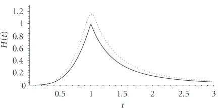
Figure 2.1. Approximative graphic of the functionsu(t,x) (dotted line) andH(t) (solid line).
Theorem2.1 (local positivity onRd). There exists a positive functionH(t)such that for
anyt >0andR >0the following bound holds true for all continuous nonnegative solutions
uto (2.1) withmc< m <1:
inf x∈BR(x0)
u(t,x)≥MRx0H t tc
. (2.3)
FunctionH(η)is positive and takes the precise form
H(η)=
⎧ ⎨ ⎩Kη
−dϑ forη≥1,
Kη1/(1−m) forη≤1. (2.4)
The characteristic time is given by
tc=CMR1−mR1/ϑ. (2.5)
ConstantsC,K >0depend only onmandd.
Figure 2.1gives an idea of the positivity result, in particular the change of the behavior of the general lower profile as a function of time. It shows the importance of the critical timetc. For the sake of simplicity, we considertc=1.
Proof. We skip the proof of this result, given in [5], since it is similar to the proof of the problem posed in a bounded domain, that we will present inTheorem 2.5; that case which presents the extra difficulty caused by the phenomenon of extinction in finite time.
Instead, we concentrate on a number of observations.
(1)Characteristic time.Notice thattcis an increasing function ofMRandR. This is in contrast with the porous medium casem >1 where it can be shown thattcdecreases with MR(see, e.g., [8] or [3, Chapter 4]).
(2)Minimax problem.Suppose that we want to obtain the best of the lower bounds
whentvaries. This happens fort/tc≈1 and the value is
utc, 0
≥C3MRR−d, (2.6)
(3) The behavior ofH is optimal in the limitst 1 andt≈0 as the Barenblatt so-lutions show. If we perform the explicit computation for the Barenblatt solution in the worst case where the mass is placed on the border of the ballBR0, it gives (see (2.8))
Ꮾ(0,t)= M
2ϑ R t1/(1−m)
b1t2ϑ+b2tc2ϑ
1/(1−m). (2.7)
The consideration of the Barenblatt solutions as an example leads us to examine what is the form of the positivity estimate when we move far away from a ball in space. Indeed, we can get a global estimate by carefully inserting a Barenblatt solution with small mass below our solution. Let us recall that the Barenblatt solution of massM is given by the formula
Ꮾ(t,x;M)= t1/(1−m)
b1t2ϑ/M2ϑ(1−m)+b2|x|2
1/(1−m), (2.8)
and also that
tc=CMR(1−m)R1/ϑ. (2.9)
The following theorem can be viewed as a weak global Harnack principle, since it leads to the global Harnack principle, which will be derived in the next section. Notice that the parameters of the Barenblatt subsolution have a different form in the two casest≥tcand 0< t < tc.
Theorem2.2 (global positivity inRd). (I)There existτ1∈(0,t
c)andMc>0such that for
allx∈Rdandt≥t c,
u(t,x)≥Ꮾt−τ1,x;Mc
, (2.10)
whereτ1=λtcandMc=kMRfor some universal constantsλ,k >0which depend only onm
andd.(II)For any0< ε < tc, the global lower bound is valid fort≥ε,
u(t,x)≥Ꮾt−τ(ε),x;M(ε), (2.11)
withτ(ε)=λεand
M(ε)= ε tc
1/(1−m)
Mc=k1 ε R1/ϑ
1/(1−m)
. (2.12)
Proof. The proof presented here has been taken from [5]. The main result is the first, the point of stating (II) is to have an estimate for small times (with a smaller time shift) at the price of having a subsolution with smaller mass. Let us point out that the last constant k1=kC−1/(1−m). We divide the proof in a number of steps; the proof of (I) consists of steps (i)–(iii). (i) Let us first argue forx∈BR(0) at timet=tc. As a consequence of our local estimate (2.1) att=tc, one gets
utc,x
≥KMR
for all|x| ≤R. Hence, (2.10) is implied in this region by the inequality
KMR Rd ≥Ꮾ
tc−τ1,x;Mc
=
tc−τ1
1/(1−m)
b1
tc−τ1
2ϑ
/Mc2ϑ(1−m)+b2|x|2
1/(1−m). (2.14)
Now we chooseτ1=λtcwith a certainλ∈(0, 1). We putμ=1−λ∈(0, 1) so thattc−τ1= μtc. With this choice, (2.14) is equivalent to
b1
μtc
2ϑ
M2cϑ(1−m)
+b2|x|2≥ Rd(1−m)μtc M1−m
R K1−m
(2.15)
puttingx=0 and using the value oftc, it is implied by the condition
Mc=kMR, k≤b11/(2ϑ(1−m))K1/2ϑ(μC)d/2. (2.16)
(ii) We now extend the comparison to the region|x| ≥R, again at timet=tc. We take as a domain of comparison the exterior space-time domain
S=τ1,tc
×x∈Rd:|x|> R. (2.17)
Both functions in estimate (2.10) are solutions of the same equation, hence we need only to compare them on the parabolic boundary. Comparison at the initial timet=τ1is clear sinceB(tc−τ1,x;Mc) vanishes. The comparison on the lateral boundary where|x| =R andτ1≤t≤tcamounts to
KMR Rd
t tc
1/(1−m) ≥
t−τ1
1/(1−m)
b1
t−τ1
2ϑ
/Mc2ϑ(1−m)+b2R2
1/(1−m). (2.18)
Raising to the power (1−m) and using the value oftc, we get
K1−mt R2C ≥
t−τ1 b1
t−τ1
2ϑ
/Mc2ϑ(1−m)+b2R2
, (2.19)
or
K1−mb1
t−τ1
2ϑ
M2cϑ(1−m)
+K1−mb
2R2≥ 1−τ1 t
R2C. (2.20)
If we have fixedτ1as before and if we defineMc=kMR withk=k(m,d) small enough, this inequality is true forτ1≤t≤tc. (iii) Using now the maximum principle inS, the proof of (2.10) is thus complete fort=tc in the exterior region. Since the comparison holds in the interior region by step (i), we get a global estimate att=tc. (iv) We now prove part (II) of the theorem. We only need to prove it att=ε. We recall thatλandMc are as defined in part (I). We know that
Using the B´enilan-Crandall estimate, we have for 0< t < tc
u(t,x)≥utc,x
t1/(1−m) tc1/(1−m)
, (2.22)
together with the above estimate (2.10), we can see that
u(t,x)≥utc,x
t1/(1−m) tc1/(1−m)
≥t1/(1−m) t1c/(1−m)
Ꮾtc−τ1,x;Mc
=t1/(1−m) tc1/(1−m)
μtc1/(1−m)
b1
μtc2ϑ/Mc2ϑ(1−m)+b2|x|2
1/(1−m)
= (μt)1/(1−m) b1(μt)2ϑ/M2ϑ(1c −m)t2ϑt−c2ϑ+b2|x|2
1/(1−m)
=Ꮾ μt,x;Mct 1/(1−m)
tc1/(1−m)
=Ꮾt−τ,x;Mc(t)
(2.23)
once one letst−τ=μtandMcas above. The proof of (2.11) is thus complete.
A consequence of this result is the following lower asymptotic behavior that is peculiar of the FDE evolution.
Corollary2.3. Under the same hypothesis ofTheorem 2.2,
lim inf
|x|→∞ u(t,x)|x|
2/(1−m)≥c(m,d)t1/(1−m). (2.24)
The constantc(m,d)=(2m/ϑ(1−m))1/(1−m)of the Barenblatt solution is sharp.
This result has been proved by Herrero and Pierre (see [9, Theorem 2.4]) by similar methods. Here, it easily follows from the estimates of Theorem 2.2which provides an exact lower bound for all times, not only for large times.
Remarks 2.4. (1) In order to complement the previous lower estimates, let us review what is known about estimates from above. These depend on the behavior of the initial data as|x| → ∞. Recall only that constant data produce the constant solution that does not decay. Under the decay assumption on the initial datumu0∈L1loc(Rd)
|y−x|≤|x|/2
u0(y)dy=O
|x|d−2/(1−m) as|x| −→ ∞, (2.25)
it has been proved by entirely different methods in [1] that
lim
|x|→∞u(t,x)|x|
2/(1−m)≤c(m,d)(t+S)1/(1−m), (2.26)
an exact decay at infinity,u0∼a|x|−2/(1−m), we have more
lim
|x|→∞u(t,x)|x|
2/(1−m)=C(t+S)1/(1−m), (2.27)
with C=2m/ϑ(1−m) and S=a1−m/C, and this cannot be improved as the delayed Barenblatt solutions show. Moreover, there exists at0such thatu1−mis convex as a func-tion ofxfort > t0, compare [10].
(2) In comparison with the upper bounds, we have shown that global lower estimates need a time shiftτ(in the other direction, explicitly calculated), but in the limit we can put τ=0, as one can see above. Moreover, the behavior at infinity is independent of the mass (a fact that is false for the heat equation), hence all Barenblatt solutions with different free constantb1behave in the same way in the limit as|x| → ∞, compare [1].
(3) We can also get better results if we consider radially symmetric initial data (always in our range of parametersmc< m <1), compare [11].
2.2. Local and global positivity estimates on domains. In this section, we will prove local positivity estimates (weak Harnack) and elliptic Harnack inequalities for the fast diffusion equation in the range (d−2)+/d=mc< m <1 in a Euclidean domainΩ⊂Rd,
ut=Δ
um inQ=(0, +∞)×Ω, u(0,x)=u0(x) inΩ, u(t,x)=0 fort >0,x∈∂Ω,
(2.28)
whereΩ⊂Rd is an open-connected domain with sufficiently smooth boundary. Since we are interested in lower estimates, by comparison, we may assume thatΩis bounded without loss of generality. In the case of bounded domains, an extra difficulty appears: the extinction in finite time, for example, there exists a timeT >0 such thatu(t,x)≡0 for any t≥Tandx∈Ω. In the proof ofTheorem 2.5, we prove a lower bound for such extinction time in terms of the volume of the domain. This will in particular show that in the case of the wholeRd, solutions do not extinguish in finite time. This is the intrinsic positivity result that shows in a quantitative way that solutions are positive for all (x,t)∈Q. In the result, we fix a pointx0∈Ωand consider different ballsBR=BR(x0) withR >0, included inΩ. It is a version ofTheorem 2.1in the case of the mixed Cauchy-Dirichlet problem on domains.
Theorem2.5 (local positivity on domains). Letube a continuous nonnegative solution to (2.28), withmc< m <1. There exist times0< tc∗< Tc≤T, whereTis the finite extinction
time, and a positive functionH(t)such that for anyt∈(0,Tc)andR >0such that
R≤Λdistx0,∂Ω, (2.29)
the following bound holds true:
inf
x∈BRu(t,x)≥MRH t t∗
c
1.2 1 0.8 0.6 0.4 0.2 0
0.5 1 1.5 2 2.5 3
t
H
(
t
)
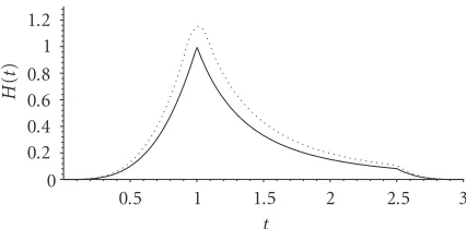
Figure 2.2. Approximative graphic of the functionsu(t,x) (dotted line) andH(t) (solid line).
whereMR=MR/Rd,MR=
BRu0(x)dx. FunctionH(t)is positive and takes the precise form
H(η)=
⎧ ⎪ ⎨ ⎪ ⎩
Kη−dϑ for1≤η≤Tc t∗
c ,
Kη1/(1−m) forη≤1. (2.31)
The times0< t∗c ≤Tc≤Tare given by
tc∗=τc(2R)1/dϑM1R−m, Tc=τc
distx0,∂Ω
−2RMR1−m.
(2.32)
ConstantsC,K,τc,τc,Λ>0depend only ondandm.
Figure 2.2gives an idea of the positivity result, in particular the change of the behavior of the general lower profile, in function of time, showing the importance of both the lower critical timetcand the upper critical timeTc. For the sake of simplicity, we considertc=1 andTc=2.5, while the extinction time is taken asT=3.
Proof. The proof presented here has been taken from [5]. It is a combination of several steps. Without loss of generality, we assume thatx0=0. Different positive constants that depend onmanddare denoted byCi. The precise values we get forC,K,τc,τc, andΛ are given at the end of the proof.
Reduction.By comparison, we may assume that supp(u0)⊂BR(0). Indeed, a general u0≥0 is greater thanu0η,ηbeing a suitable cutofffunction compactly supported inBR and less than one. Ifvis the solution of the fast diffusion equation with initial datau0η (existence and uniqueness are well known in this case), we obtain
BRu(0,x)dx≥
BRu0(x)η(x)dx=MR (2.33)
and if the statement holds true forv, then
inf
x∈BRu(t,x)≥xinf∈BRv(t,x)≥H t tc
Lower bounds on the extinction time.In order to get a lower bound for the extinction time in terms of local mass information, we use a property which can be labeled as weak conservation of mass, and has been proved in [9, Lemma 3.1]. It reads: for anyR,r >0 ands,t≥0, one has
B2R
u(s,x)dx≤C3
B2R+r
u(t,x)dx+ |s−t| 1/(1−m)
r(2−d(1−m))/(1−m)
. (2.35)
Now lettingt=T, so thatu(T,x)=0, ands=0 so thatB2Ru(0,x)dx=MR, we get
T≥MR1−mr1/ϑ C13−m
≥MR1−m
dist(0,∂Ω)−2R1/ϑ C13−m
, (2.36)
sincer∈(0, dist(0,∂Ω)−2R).
A priori estimates.The second step again is similar to the analogous step in the proof ofTheorem 2.1, so we will omit the details. We rewrite the well-known smoothing effect (see, e.g., [3]), after an integration overB2bR, in the form
B2b R
u(t,x)dx≤C2M2RϑRdt−dϑ, (2.37)
sinceu0is nonnegative and supported inBR. HereC2=C12bdωd.
Integral estimate.Again in this step we are going to use the estimate (2.35). We lets=0 and we rewrite it in a form more useful to our purposes (remember thatM2R=MRsince u0is supported inBR):
B2R+r
u(t,x)dx≥MR C3 −
t1/(1−m)
r1/θ(1−m), (2.38)
we now remark thatrandRare such thatB2R+r⊂Ω.
Aleksandrov principle.The fourth step consists in using the well-known reflection prin-ciple in a slightly different form (seeProposition A.1and formula (A.5) in the appendix for more details). This principle reads
B2R+r\B2b R
u(t,x)dx≤Adrdu(t, 0), (2.39)
whereAdandb=2−1/dare chosen as in (A.5) in the appendix, and one has to remem-ber the conditionr≥(2(d−1)/d−1)2R.
We now put together all the previous calculations:
B2R+r
u(t,x)dx=
B2b R
u(t,x)dx+
B2R+r\B2b R
u(t,x)dx
≤C2M2RϑRdt−dϑ+Adrdu(t, 0).
(2.40)
This follows by (2.37) and (2.39). Now we are going to use (2.38) to obtain
MR C3 −
t1/(1−m) r1/θ(1−m)≤
B2R+r
u(t,x)dx≤C2MR2ϑRd
And finally we obtain
u(t, 0)≥ 1 Ad
MR C3 −
C2MR2ϑRd tdϑ
1 rd −
t1/(1−m) r2/(1−m)
= 1 Ad
A(t) rd −
B(t) r2/(1−m)
. (2.42)
Now we would like to obtain the claimed estimate for t > tc∗. To this end, we seek whetherA(t) is positive:
A(t)=MR C3 −C2
M2RϑRd
tdϑ >0⇐⇒t >
C3C2
1/(dϑ)
M1R−mR1/ϑ=tc∗. (2.43)
Now we have to check ift∗c ≤T. By (2.36), one knows that a sufficient condition is that tc∗≤Tc=Cm3−1MR1−m[dist(0,∂Ω)−2R]1/ϑ≤T, that is,
R≤ dist(0,∂Ω) 2 +C13−m+1/dϑC12/dϑ
. (2.44)
Now, assuming thatt∈(tc∗,Tc) is temporarily fixed, we optimize the function
f(r)= 1 Ad
A(t) rd −
B(t) r2/(1−m)
(2.45)
with respect tor=r(t)∈(0, dist(0,∂Ω)−2R) and we obtain that it attains its maximum inr=rmax(t):
rmax(t)=
2
d(1−m)
ϑ(1−m) tϑ
MR C3 −
C2MR2ϑRd tdϑ
−ϑ(1−m)
. (2.46)
At this point, it is necessary to check the conditions
2(d−1)/d−12R < r
max(t)<dist(0,∂Ω)−2R. (2.47)
To this end, it is useful to get a simpler parametrization of the time interval (tc∗,Tc), indeed
tα=αt∗c =α
C3C2
1/(dϑ) M1−m
R R1/ϑ (2.48)
maps the time interval (tc∗,Tc) into (1,αc), where
αc=Tc t∗
c =C 1−m+1/dϑ 3 C21/dϑ
dist(0,∂Ω) R −2
, rmax tα = 2
d(1−m)
ϑ(1−m)
C13−m+1/dϑC12/dϑ α ϑ
1−α−dϑϑ(1−m)R.
(2.49)
Now optimizing this function with reflect toα∈(1,αc) will lead to the value
and in order to guarantee the fact thatαmin≤αc, we impose the condition
R≤ dist(0,∂Ω)
2 +1 +ϑd(1−m)C31−m+1/dϑC12/dϑ
ϑ. (2.51)
Moreover, it is tedious but straightforward to verify that
2(d−1)/d−12R < r max
tαc
≤distx0,∂Ω
−2R, (2.52)
the first inequality becomes nothing else but a lower bound on the constantsC2andC3, but since they are constants used in upper estimates, they can be chosen arbitrarily large. The second inequality is guaranteed by the hypothesisR≤Λdist(0,∂Ω). Now going back to the standard time parametrization, we proved that
frmax(t)
=Ad
d(1−m)2ϑ−1 22ϑϑ
1 C3−C2
M2ϑ−1 R Rd
tdϑ
2ϑM2ϑ R
tdϑ >0 (2.53)
for allt∈(tαmin,Tc)⊂(tc∗,T). We thus found the estimate
u(t, 0)≥Ad
d(1−m)2ϑ−1 22ϑϑ
1
C3−C2
MR2ϑ−1Rd tdϑ
2ϑM2ϑ R
tdϑ =K1A(t) MR2ϑ
tdϑ , (2.54)
a straightforward calculation shows that the function
A(t)= 1 C3−C2
MR2ϑ−1Rd tdϑ
2ϑ
(2.55)
is nondecreasing in time, thus ift≥tαmin,
A(t)≥Atαmin
=
1−1 +ϑd(1−m)−dϑ 2C3
2ϑ
(2.56)
and finally we obtain
u(t, 0)≥K1A(t)M 2ϑ R tdϑ ≥K1A
tαmin
MR2ϑ
tdϑ . (2.57)
So we proved that
u(t, 0)≥KM 2ϑ R
tdϑ (2.58)
fort∈(tαmin,Tc), with
K= Ad
2C3
2ϑ
d(1−m)2ϑ−1 22ϑϑ
1−1 +ϑd(1−m)−dϑ2ϑ. (2.59)
in some pointxm∈BR, so that infx∈BRu(t,x)=u(t,xm), then one can apply (2.58) to this point and obtain
ut,xm≥KM 2ϑ 2R
xm
tdϑ (2.60)
fortαmin(xm)< t < Tc(xm)< T. Since the pointxm∈BR(0), then it is clear thatBR(0)⊂ B2R(xm)⊂B4R(0) and this leads to the equality
M2R
xm
=MR(0)=M4R(0) (2.61)
sinceMρ(y)=Bρ(y)u0(x)dx, supp(u0)⊂BR(0) andu0≥0. These equalities will imply then that the times
tαmin
xm=1 +ϑd(1−m)C3C2
1/dϑ
(2R)1/ϑM 2Rxm
=1 +ϑd(1−m)C3C21/dϑ(2R)1/ϑMR(0)=tmin∗ (0)≥tαmin(0),
(2.62)
Tc
xm
=C3m−1
dist(0,∂Ω)−4R1/ϑM21−Rm
xm
=Cm−1 3
dist(0,∂Ω)−4R1/ϑM1−m
R (0)≤Tc(0).
(2.63)
Thus, we have found that
inf
x∈BR(0)u(t,x)=u
t,xm
≥KM 2ϑ R
xm
tdϑ =K M2ϑ
R (0) tdϑ =K
t∗dϑ min(0)
tdϑ M2ϑ
R (0) t∗dϑ
min(0)
(2.64)
fortc∗=t∗min(0)< t < Tc(0)< T, which is exactly (2.30).
The last step consists in obtaining a lower estimate when 0≤t≤t∗c.
To this end, we consider the fundamental estimate of B´enilan and Crandall [12]
ut(t,x)≤(1u(t,x)−m)t. (2.65)
This easily implies that the function
u(t,x)t−1/(1−m) (2.66)
is nonincreasing in time, thus, for anyt∈(0,tc), we have
u(t,x)≥utc∗,xt 1/(1−m)
tc∗1/(1−m)
. (2.67)
The values of the constantsKandCare given by
K= Ad
2C3
2ϑ
d(1−m)2ϑ−1 22ϑϑ
1−1 +ϑd(1−m)−dϑ2ϑ 2dC3C21 +ϑd(1−m) ,
C=C31−m+1/dϑC21/dϑ,
τc=1 +ϑd(1−m)C3C21/dϑ,
τc= 1 C1−m
3 ,
Λ=min
1 (2 +C),
1
2 +1 +ϑd(1−m)Cϑ
.
(2.68)
The proof is complete.
Global positivity on domains. The global positivity in this setup has been proved first by DiBenedetto et al. [7] in the form of the global Harnack principle that we will discuss in the following section.
3. Global Harnack principle on the whole space and relative error estimates
Under a further control on the initial data, we can transform the local Harnack princi-ple into a global version. Theglobal Harnack principle, which is the natural extension of Harnack inequalities to a global point of view, is indeed nothing else than aglobal sharp upper and lower boundin terms of a Barenblatt solution shifted in time and possibly with different mass. The range of the parametermis alwaysmc< m <1. We recall thatbi,λ1, k1, andCiare constants that depend only onmandd, while the rest of the parameters depend also on the data as expressed.
Theorem3.1 (global Harnack principle). Letu0∈L1(Rd),u0≥0, and
u0(x)|x|2/(1−m)≤A (3.1)
for|x| ≥R0. Then, for any timeε >0, there exist constantsτ1,τ2,M1, andM2, such that for
any(t,x)∈(ε,∞)×Rd, the following upper and lower bounds hold:
Ꮾt−τ1,x;M1
≤u(t,x)≤Ꮾt+τ2,x;M2
, (3.2)
where τ1=λ1ε,τ2=τ(ε,A,ts), M1=M(ε)as given in Theorem 2.2, and M2=k2(ε,A, τ2)M∞, while
tc=CMR1−mR1/ϑ, ts=C5M∞1−mR10/ϑ. (3.3)
Proof. The detailed proof can be found in [5]. It is based on a quite delicate analysis of the properties of the solution and the size of the Barenblatt solutions in different parts of the space-time domain. Convenient parabolic comparisons are then used to arrive at the
Asymptotic behavior and relative error estimates inRd. The second author has proved in [1] the so-called relative error estimates (REE) for the FDE in the same range of parame-ters, namely,
lim t→∞
u(t,·Ꮾ(t,)−Ꮾ·;M)(t,·;M)
∞=0, (3.4)
whereᏮis the Barenblatt solution with the same mass (the result is independent of a possible shift in time or space). This is related to ourTheorem 3.1as follows: for every ε >0, we can find a Barenblatt solution with massM1(ε)< M∞ and another one with
massM2(ε)> M∞that serve as lower bound, respectively, upper bound for the solution
for all timest≥ε. It is clear from the maximum principle thatM1(ε) increases with time whileM2(ε) decreases. The asymptotic result says that
lim
ε→∞M1(ε)=εlim→∞M2(ε)=M∞. (3.5)
Theorem 3.1adds to this asymptotic statement a more precise quantitative information that is valid not only for large times, but also for arbitrary small times. The solution thus inherits positivity and boundedness properties directly from the Barenblatt solutions that serve as upper and lower bounds from the very beginning. Usually, it is said that the Barenblatt solution of the nonlinear equations is a “poor cousin” of the fundamental solution of the heat equation since there is no representation formula as in the linear case. The above results show that in the good fast diffusion rangemc< m <1, it is a stronger model in some respects. Thus, a consequence of this powerful global Harnack principle, obviously valid for the Barenblatt solutions, is that the behavior at infinity (i.e., for|x| → ∞and/ort→ ∞) of the Barenblatt solution is always the same, independent of the mass. This uniformity property is not shared by the heat equation nor by the porous medium equation and it shows how much more effectively the fast diffusion process regularizes the initial data.
Different behavior in the casesm∈(mc, 1). In the above considerations, it is essential that the range of parameters ismc< m <1, since whenm∈(mc, 1), different phenomena hold. We refer to [3] for a detailed and exhaustive exposition and as a source for more complete bibliography. Let us discuss here the question of possible uniform lower bounds. The following result is proved in [5].
Proposition3.2. Locally uniform positivity estimates and a posteriori any kind of Harnack inequalities are false for general initial data.
This quite simple example shows that the range of parameters we consider in this paper is optimal from below, if we want the initial datumu0to be as general as possible.
Let us now comment that the results discussed above have been motivated by similar properties of the heat equation flow. It has to be noted that there are slight differences in favor of the fast diffusion case. Indeed, if one considers as initial datumu0=δy, then it is easy to see that the shifted fundamental solution of the linear heat equation
Ey(t,x)=(4πt)−d/2e−|x−y| 2/t
does not satisfy the condition
c1E0(t,x)≤Ey(t,x)≤c2E0(t,x) (3.7)
for some universal constantsci>0, which is, however, satisfied by the Barenblatt solutions ifmc< m <1.
4. Global Harnack principle on bounded domains
In this section, we will enlarge a bit the range of the parameterm, namely, we will consider
(d−2)+
d+ 2 =ms< m <1, (4.1)
withms≤mc(note thatmsis the inverse of the usual Sobolev exponent). Passing now from the local to the global point of view, we should mention that the global Harnack principle in the case of bounded domains has been proved by DiBenedetto et al. [7]. They investigate some regularity properties of the FDE problem posed on bounded domains. We quote hereafter their [7, Theorem 1.1] for convenience of the reader and since it will be used in the sequel, for its relation with the fine asymptotic behavior, near the extinction time.
Theorem4.1 (global Harnack principle on bounded domains) [7]. For anyε∈(0,T), there exist constantsλ,Λdepending only upond,m,u01+m,∇um02,diam(Ω),∂Ω, and ε, such that for all(t,x)∈(0,T)×Ω,t > ε
λdist(x,∂Ω)1/m(T−t)1/(1−m)≤u(t,x)≤Λdist(x,∂Ω)1/m(T−t)1/(1−m). (4.2)
This global Harnack principle also gives further regularity of the solutions (namely space analyticity and time H¨older continuity), and holds on bounded domains depending on some further global regularity of the initial datum. The difference between theRdcase and the bounded domain case is that in the case of whole spaceRd the general solution u(x,t) is estimated from above and from below in terms of the Barenblatt solution, while in the case of a bounded domain, it is bounded betweend(x)1/m(T−t)1/(1−m), which is essentially the solution obtained by separation of variables.
We conclude this topic section by saying that the global version of the elliptic Harnack inequality is the global Harnack principle, that is, nothing more than an accurate lower and upper bound with the same “comparison function,” both in the case of the whole space and in the case of bounded domains. As far as we know, it is an interesting open problem to find such global principle in unbounded domains.
5. Convergence in relative error on a domain
boundary value problem
ut=Δum in (0, +∞)×Ω, u(0,x)=u0(x) inΩ, u(t,x)=0 fort >0, x∈∂Ω
(5.1)
posed in a bounded connected domainΩ⊂Rdwith sufficiently smooth boundary; as we have said,ms< m <1. We assume that the initial datau0is bounded and nonnegative. We recall that the above problem possesses a unique weak solutionu≥0, that is, defined and positive for some time interval 0< t < Tand vanishes at a timeT=T(m,d,u0)>0, which is called the (finite) extinction time, compare [13,7]. Note that the conditions on the initial data can be relaxed intou0∈Lp(Ω) for somep > pcwherepc=max{1,d(1− m)/2}in view of theLp–L∞smoothing effect
u(t)
∞≤Cm,du0γpt−α for anyt >0, (5.2)
valid forp > pcwithγ,α >0 depending only onm,d,p(see [3] for further details on this issue).
The asymptotic profiles and the associated elliptic problem. We want to investigate the pre-cise behavior of the solution near the extinction time. For this purpose, it is convenient to transform the above problem by the known method of rescaling and time transforma-tion. If we put
u(t,x)=(T−t)1/(1−m)w(τ,x), τ=log T (T−t)
, (5.3)
then, problem (5.1) is mapped into
wτ=Δwm+1−w
m in (0, +∞)×Ω, w(0,x)=T−1/(1−m)u0(x) inΩ,
w(τ,x)=0 forτ >0,x∈∂Ω.
(5.4)
The transformation can also be expressed as
w(τ,x)=u
T−Te−τ,x
Te−τ1/(1−m) , (5.5)
problem
−ΔSm= 1
1−mS inΩ, S(x)=0 forx∈∂Ω,
(5.6)
wherems< m <1 andΩare as before.
We will prove that the solutions of problem (5.4) have asω-limits nontrivial solutions of problem (5.6), and also that the convergence takes place in the weighted uniform sense that we will explain next. Every solutionSto the elliptic problem produces a separable solutionᐁof the original FDE of the form
ᐁ(t,x)=S(x)(T−t)1/(1−m) (5.7)
which corresponds to the initial datumᐁ(0,x)=T1/(1−m)S(x). In this context, we can fix Tat will, and we will writeᐁT for definiteness.
The elliptic problem. The question of existence, regularity, and uniqueness for the Dirich-let elliptic problem is well understood in its basic features, in the range of parameters under consideration.
Existence of positive classical solutions. If 0< m <1 ford≤2 or if (d−2)/(d+ 2)=ms< m <1 ford≥3, then there exist positive classical solutions to equation (5.6) (see, e.g., [13] and references quoted therein, and also [7]).
Uniqueness. In the supercritical casem > msthat we consider,the geometry ofΩplays a
role in the uniqueness problem. Indeed, ifd=1 or ifd≥2 andΩis a ball, then the solution is unique (see [14]). Moreover, ifd≥2 andΩis an annulus, then the solution is unique in the class of positive radial solutions (see [15]). However, there are cases in which the solution is not unique, see; for example, [16,15].
Regularity and boundary behavior. Since the solutions of problem (5.6) are stationary solutions of problem (5.1), estimates (4.2) give us the following estimates for the behavior ofS:
λd(x)1/m≤S(x)≤Λd(x)1/m. (5.8)
Dynamical system approach:ω-limits. For convenience of the reader, we introduce now some basic ideas from the dynamical system approach. Basically, this approach consists of viewing the solution as an orbit in a functional space and considering the points to which it accumulates as time goes to infinity. We suggest to the interested reader the books [17,18] for this approach. Note that the approach is applied to the rescaled solutions that have nontrivial asymptotics.
Definition 5.1. The positivesemiorbitof a solutionw(τ,x) starting at timet0if the family
γw;τ0
=w(τ) :τ≥τ0
, (5.9)
Hopefully,Xwill be a Banach space or a closed convex subset thereof. With the previ-ous estimates, the semiorbit is a relatively compact subset ofLp, with 1≤p≤ ∞, which can be taken asX, since the semiorbit is uniformly bounded inL∞. In any case, for every sequenceτj, there is a subsequence along which
wτjk−→f inLpstrong, withp∈[1,∞]. (5.10)
Definition 5.2. The set of all possible limits of a semiorbit along sequencesτj→ ∞is calledω-limitof the orbit
ᏸ(w)=f ∈Lp:∃τj−→ ∞,wτj−→f inLpstrong. (5.11)
An alternative way of writing this definition is
ᏸ(w)=
τ>0
τ≥τ0
γ(w;τ), (5.12)
where the overline denotes the closure.
It is well known that theω-limit is a closed and connected set inX. We now revisit the well-known result by Berryman and Holland [13] who proved convergence inW1,2 by similar methods, based on Lyapunov functional techniques. Our first result is a little improvement in the sense that in [13] the authors do not prove uniform convergence for dimensions higher than 1.
Theorem 5.3 (uniform convergence to the ω-limit) [4]. The ω-limit set ᏸ(u) of a rescaled solution of the parabolic problem (5.1) is contained in the set of a solution of the elliptic problem (5.6) and the convergence takes place uniformly inΩast→T−.
Remark 5.4. In case the solution of the elliptic problem is unique, theω-limit consists of a single pointᏸ(w)=Sgiven by such unique solution. In this case, the convergence is unconditioned (i.e., ast→T), since along any sequencetj→T(i.e.,τj→ ∞), we have convergence to the same pointᏸ(w)=S, in allLp(Ω) spaces withp∈[1,∞].
Relative error convergence. We are now ready to address the main issue of this section, that is, the relative error convergence estimates (REC) which are nothing else but uniform estimates ast→T−of the quotient of the solution to the FDEudivided by a separable solutionᐁTto the same problem,Tbeing the finite extinction time. The formulation of the result depends on whether the elliptic problem has multiple solutions so that the ω-limit setᏸ(w) ofTheorem 5.3may consist of many points, or the solution to this problem is unique. The general result is as follows.
Theorem5.5. Letube the solution to the problem (5.1). Then,
lim t→T−Sinf∈ᏸ
S(·)(Tu(t,−t)·)1/(1−m)−1
L∞(Ω)=0, (5.13)
This type of convergence is what we calluniform relative-error convergence(REC for short), and it is our main contribution to the subject of fine asymptotics. To understand better the meaning of this terminology, it will be convenient to introduce the weighted distance to the set
d∞(f,)=inf
S∈
S(f(··))−1
L∞(Ω). (5.14)
This peculiar distance (which gives a topology strictly finer than the standardL∞norm) is zero if and only if f is a point of.Theorem 5.5says that the relative distance between the trajectory f(t)=u(t)(T−t)−1/(1−m)and theω-limit set,
d∞ u(t)
(T−t)1/(1−m),
−→0, ast−→T, (5.15)
is going to zero uniformly in space variables ast→T. Loosely speaking, taking into ac-count the behavior of bothuandSnear the boundary, what we say is that, ifd(x) denotes distance to the boundary, then
u(t,x)−S(x)(T−t)1/(1−m)
d(x)(T−t)1/(1−m) −→0 (5.16)
converges to zero uniformly inx∈Ωast→T. We also state a particular case of the above theorem, the case where the Dirichlet elliptic problem (5.6) has a unique positive classical solutionS(x). In that case, the result takes the simpler form.
Theorem5.6. Letube the solution to problem (5.1). Then,
lim t→T−
ᐁ(t,u(t,··))−1
L∞(Ω)=0, (5.17)
whereᐁis the separable solution (5.7) of the form
ᐁ(t,x)=S(x)(T−t)1/(1−m). (5.18)
Let us now choose a parametrization of the setof solutions to the elliptic problem (5.6),= {Sα}α∈A. Then,ᏸ(u)⊂and both sets are possibly not equal.ᏸinherits the parametrization of, thus, for anyusolution to the problem (5.1), there exists anA= A(u)⊂Asuch that
ᏸ(u)=Sα
α∈A. (5.19)
It is worth noting that when theω-limit consists of one point, that is, when the elliptic problem (5.6) possesses a unique solution, things are simpler and the parametrization below is trivial, that is, the setA=A= {α1}, thus we will omit the subindexesαwhen no confusion is feared.
Corollary5.7. With the same hypothesis as inTheorem 5.5, for anyε >0there existtε>0
and a functionα(t)∈A, defined for anytε< t < Tsuch that
u(t)S
α(t)−1
∞≤ε, for anytε< t < T. (5.20)
This corollary is important since it allows to prove elliptic Harnack inequality near the extinction time, also in the case when the ω-limit set consists of many points, as we will see in a subsequent section. This will show also that the regularity properties of the solution are somehow independent of the exact profile of the solution close to the extinction time.
Comments. The above results improve on the celebrated result of Berryman and Holland [13], where it was shown that the asymptotic profile for the solution to (5.1) is given by the separable solutionᐁ, but convergence was proved only for some special classes of initial data and in some Sobolev spaces; that convergence in general does not imply uniform convergence up to the boundary. Our result of convergence in relative error is stronger than uniform convergence because of the fine behavior near the boundary; moreover, it easily implies elliptic Harnack inequalities near finite extinction timeT.
It is also worth noticing that the convergence result can be viewed as a concrete S-theorem, in the spirit of [17], applied to the problem under consideration. The proof borrows the main lines of the proofs of the same result for the PME as done, for example, in [2].
Let us also note that the convergence in relative error cannot be true for obvious rea-sons when the profiles have moving free boundaries, like in the porous medium case or its rescaled version (nonlinear Fokker-Planck equation), and the problem is posed in free space. This is due to the fact that the interfaces do not match exactly, so that the quotient u/ᐁmay be infinite. As a final note on this issue, let us point out that our REC result shows convergence in time to theω-limit, but the question of establishing precise rates is not investigated. This is a natural further question that deserves attention.
6. Harnack inequalities
We finally come to one of the most important aims of this paper. We want to show how an intelligent combination of direct and reverse smoothing effects implies easily an optimal Harnack inequality, whose form changes in time.
As a precedent, DiBenedetto and Kwong proved an intrinsic Harnack inequality (see [19, Theorem 2.1]):there exist constants0< δ <1andC >1depending ondandmsuch that for every pointP0=(t0,x0)∈QT,QT=(0,T)×Ω,
inf x∈BRu
t0+θ,x
≥Cut0,x0
(6.1)
providedu(t0,x0)is strictly positive and
t0−τ,t0+τ
×BR
x0
⊂QT, τ=u
t0,x0
1−m
The constantθ=δτdepends on the positive value ofuatP0. It is a local property and thus it holds both for the case of the whole space and for the domain case. Our local pos-itivity results, Theorems2.1and2.5, support quantitatively the above intrinsic Harnack inequality, proving its validity in another aspect.
We will present intrinsic and elliptic forms of the Harnack inequality. We can say that the intrinsic Harnack inequality, which compares values of the solution in different times, is the only Harnack possible for small times, while for intermediate times, the elliptic Harnack inequality seems to be the best one: it is stronger, since it easily implies the Intrinsic.
6.1. Harnack inequalities for the FDE onRd. We now show that the positivity result implies a full local Harnack inequality on the whole Euclidean space. We will see that once again, the critical time
tc=Cm,dMR(1−m)R1/ϑ (6.3)
plays a role, indeed, the form of the Harnack inequality changes when dealing with times smaller or larger thantc. First we deal with the case of large times, namely,t > tc: we will consideru0∈L1(Rd),u0≥0 and we let
M∞=
Rdu0(x)dx, MR=
BRu0(x)dx (6.4)
for someR >0,x0∈Rd.
Theorem6.1 (elliptic Harnack inequality). Letu(t,x)satisfy the same hypothesis as The-orem2.1. If moreoveru0∈L1(Rd), there exists a positive constantᏴ, depending only onm
anddon the ratioMR/M∞, such that for anyt≥tc(MR,R),
sup x∈BR
u(t,x)≤Ᏼinf
x∈BRu(t,x). (6.5)
If moreoveru0is supported inBR, then the constantᏴis universal and depends only onm
andd.
Proof. First we remark that the exact expression fortcis given inTheorem 2.1. The well known smoothing effect can be rewritten in an equivalent form
sup
x∈BRu(t,x)≤C
1M∞2ϑt−dϑ=C1
M∞
MR
2ϑ
MR2ϑt−dϑ. (6.6)
Using now the reverse smoothing effect whent > tc, we get
inf
x∈BRu(t,x)≥KM 2ϑ
R t−dϑ≥KC1−1
MR M∞
2ϑ sup x∈BR
u(t,x), (6.7)
that is, (6.5) withᏴ=K−1C
The above elliptic Harnack inequality holds for times larger than the critical timetc and it strongly depends on the sharp lower bounds ofTheorem 2.1, fort > tc. In the case of small times, the lower bound changes its shape and we recover the intrinsic Harnack inequality of [19] by different methods and with a little improvement: the intrinsic Har-nack inequality (6.18) holds for any positive time, namely, we have the following
Theorem 6.2 (intrinsic Harnack inequality). Let u(t,x)satisfy the same hypothesis as
Theorem 2.1, and letR >0. There exist constants0< δ <1andC >1depending onmand
dsuch that for every0< t0≤tc,
inf x∈BRu
t0+θ,x≥Cut0,x0, (6.8)
where
θ=δτ, τ=ut0,x0
1−m
R2>0. (6.9)
Proof. Let us consider the lower bound ofTheorem 2.1in the case 0< t < tc:
u(t,x)≥ t1/(1−m) tc∗1/(1−m)
ut∗c,x≥ t1/(1−m) tc∗1/(1−m)
MR2ϑ t∗c,dϑ
=C3C2
2/d(1−m)t1/(1−m)
R2/(1−m) (6.10)
since
tc∗=C3C2
1/(dϑ) M1−m
R R1/ϑ, ϑ=
1
2−d(1−m). (6.11)
We remark that we can takeC3C2>1, as remarked in the proof ofTheorem 2.2, and such intrinsic lower bound is independent ofMR, and thus ofu0. Indeed, the choices
t=t0+θ, θ=δτ, τ=u(t0,x0)1−mR2>0, (6.12)
whereδ∈(0, 1) can be chosen in such a way thatt0+δτ≤tc∗and the positivity ofτ is guaranteed by the positivity estimates. We then get
ut0+θ,x
≥C3C2
2/d(1−m)t0+θ
1/(1−m)
R2/(1−m)
>C3C2
2/d(1−m)θ1/(1−m) R2/(1−m) =C3C2
2/d(1−m)
δ1/(1−m)ut 0,x0
.
(6.13)
This concludes the proof.
the elliptic Harnack inequality. Indeed,
sup
x∈BRu(t−ω,x)≤ sup
x∈Ωu(t−ω,x)≤C1 M2ϑ
∞
(t−ω)dϑ
=C1 K
M∞
MR
2ϑ t
t−ω
dϑ MR2ϑt−dϑ
≤C1 K
M∞
MR
2ϑ t
t−ω
dϑ inf x∈BRu(t,x)
=C1 K
1 1−σ
dϑM
∞
MR
2ϑ inf x∈BRu(t,x)
(6.14)
since we tookω=σt, withσ∈[0, 1). Thus, it can be rewritten as
inf
x∈BRu(t+ω,x)≥Ᏼxsup∈BRu(t,x) (6.15)
and in particular, we can chooseσ∈[0, 1) such thatω=σt=δu(t0,x0)1−mR2=θ, as in the above intrinsic Harnack inequality (6.18).
Finally, we remark that the Harnack inequality (6.15) holds for anyσ∈[0, 1), thus it compares the infimum and supremum ofuat different times, and by the monotonicity of theL∞ norm, we can compare the supremum and infimum ofuat any two different timest1,t2∈(0,∞). This inequality is sometimes called the backward Harnack inequality, in the case of the heat equation.
Panorama. At this point, it is convenient to make a summary for the Cauchy problem
inRd. The role of the critical timet
cis to split the time axis into two parts, showing the range of validity of different Harnack inequalities and behaviors of the solutions.
(i)Small times,0< t < tc: intrinsic Harnack inequalities [19] andTheorem 6.2. The validity for all positive times is guaranteed by our local positivity result. The constants do not depend onu0. There is H¨older continuity, implied by Harnack inequalities.
(ii)Large times,t > tc: elliptic Harnack inequalities. The constant may depend on the initial datum. Elliptic Harnack inequalities imply intrinsic Harnack inequalities and H¨older continuity.
(iii)All positive times,for anyε >0 and for allt > ε: global Harnack principle that implies the convergence in relative error.
(iv)Asymptotics,t→ ∞: uniform convergence in relative error.
6.2. Harnack inequalities for FDE on a domain. In this section, we analyze the case of the mixed Cauchy-Dirichlet problem on a bounded domain. We find an extra difficulty, due to the presence of the finite extinction time. We start by recalling the result of [7], where the following rather peculiar property of the solutions of problem (2.28) is found as a consequence of the global Harnack principle on domains,
ut0,x0
≥γ0 sup
|x−x0|<R ut0,x
valid for anR >0, so small that the box
t0−τ,t0+τ
×BR
x0
⊂QT, τ=u
t0,x0
1−m
R2, (6.17)
but again the box depends on the positivity value ofuin the point (t0,x0). It resembles our elliptic Harnack inequality, but again it has to be supported by a positivity result to hold in full generality.
Analogously to what we did before, we can prove the elliptic Harnack inequality for intermediate times in the case of bounded domains. Our main result takes the form of a precise lower estimate for the values in question, and will thus ensure that such intrinsic Harnack inequality will hold for all positive times not too close to the extinction time. We also prove an elliptic Harnack inequality for intermediate times, that is, fort∈I=[tc,Tc] with 0< tc< Tc< T, wheretcandTc are computed in terms of the initial datum, which follows from our sharp result on positivity. Note that this allows to calculate explicitly all the constants. As before, we can say that our positivity results somehow “support” the results of [7], in the sense that we ensure positivity in a quantitative way, and a posteriori their result holds true for times not too close to the extinction time.
In this section, we prove intrinsic and elliptic Harnack inequalities, in the whole in-terval (0,T), in analogy to what has been done in the whole space. We point out that for times close to the extinction time, an elliptic Harnack inequality is still valid, thanks to the accurate asymptotic information given by the relative error estimates, compare Theorems 5.5and5.6.
Theorem6.4 (intrinsic Harnack inequality). Letu(t,x)andR >0satisfy the same hypoth-esis asTheorem 2.1. There exist constants0< δ <1andC >1depending onmanddsuch that for every0< t0≤tc,
inf x∈BRu
t0+θ,x≥Cut0,x0, (6.18)
where
θ=δτ, τ=ut0,x0
1−m
R2>0. (6.19)
Proof. The proof is formally the same as inTheorem 6.2.
Theorem6.5 (elliptic Harnack inequality for intermediate times). Letu(t,x)andR > 0satisfy the same hypothesis asTheorem 2.5. If moreoveru0∈L1(Ω), then there exists a
positive constantᏴ, depending only onm,d, and on the ratio
MΩ MR0
=
Ωu0(x)dx
BR0u0(x)dx
, (6.20)
such that for anytc∗< t < Tc< T,
sup x∈BR0
u(t,x)≤Ᏼ inf x∈BR0
u(t,x). (6.21)
If moreoveru0is supported inBR0, then the constantᏴis universal and depends only onm