Solutions and Green’s function of the first order linear equation with reflection and initial conditions

(1)

R E S E A R C H

Open Access

Solutions and Green’s function of the ﬁrst

order linear equation with reﬂection and

initial conditions

Alberto Cabada

*

_{and Fernando Adrián Fernández Tojo}

*_{Correspondence:}

[email protected] Departamento de Análise Matemática, Facultade de Matemáticas, Universidade de Santiago de Compostela, Santiago de Compostela, Galicia 15706, Spain

Abstract

This work is devoted to the study of the existence and sign of Green’s functions for first order linear problems with constant coefficients and initial (one point) conditions. We first prove a result on the existence of solutions ofnth order linear equations with involutions via some auxiliary functions to later prove a uniqueness result in the first order case. We study then different situations for which a Green’s function can be obtained explicitly and derive several results in order to obtain information as regards the sign of the Green’s function. Once the sign is known, optimal maximum and anti-maximum principles follow.

Keywords: equations with involutions; equations with reﬂection; Green’s functions; maximum principles; comparison principles; periodic conditions

1 Introduction

The study of functional differential equations with involutions (DEI) can be traced back to the solution of the equationx(t) =x(/t) by Silberstein (see []) in . Briefly speak-ing, an involution is just a functionf that satisfiesf(f(x)) =xfor everyxin its domain of definition. For most applications in analysis, the involution is defined on an interval ofR and in the majority of the cases, it is continuous, which implies it is decreasing and has a unique fixed point. Ever since that foundational paper of Silberstein, the study of problems with DEI has been mainly focused on those cases with initial conditions, with an extensive research in the case of the reflectionf(x) = –x.

Wiener and Watkins study in [] the solution of the equationx(t) –ax(–t) =  with ini-tial conditions. Equationx(t) +ax(t) +bx(–t) =g(t) has been treated by Piao in [, ]. In [, –] some results are introduced to transform this kind of problems with involutions and initial conditions into second order ordinary differential equations with initial conditions or first order two dimensional systems, granting that the solution of the last will be a solu-tion to the first. Furthermore, asymptotic properties and boundedness of the solusolu-tions of initial first order problems are studied in [] and [], respectively. Second order bound-ary value problems have been considered in [, –] for Dirichlet and Sturm-Liouville boundary value conditions, higher order equations has been studied in []. Other tech-niques applied to problems with reflection of the argument can be found in [–].

More recently, the papers of Cabadaet al.[, ] have further studied the case of the second order equation with two-point boundary conditions, adding a new element to the

(2)

previous studies: the existence of a Green’s function. Once the study of the sign of the aforementioned function is done, maximum and anti-maximum principles follow. Other works in which Green’s functions are obtained for functional diﬀerential equations (but with a fairly diﬀerent setting, like delay or normal equations) are, for instance, [–].

In this paper we try to answer to the following question: How is it possible find a solution of an initial problem with a differential equation with reflection? What is more, in which cases can a Green’s function be constructed and how can it be found?

Section  will have two parts. In the first one we construct the solutions of thenth order DEI with reflection, constant coefficients and initial conditions. In the second one we find the Green’s function for the order one case. In Section  we apply these findings in order to describe exhaustively the range of values for which suitable comparison results are fulfilled and we illustrate them with some examples.

2 Solutions of the problem

In order to prove an existence result for thenth order DEI with reﬂection, we consider the even and odd parts of a functionf, that is,fe(x) := [f(x) +f(–x)]/ andfo(x) := [f(x) –

f(–x)]/ as done in [].

2.1 Thenth order problem

Consider the followingnth order DEI with involution:

Lu:=

n

k=

aku(k)(–t) +bku(k)(t)

=h(t), t∈R; u(t) =c, (.)

where h∈L_loc(R), t,c,ak,bk ∈Rfork= , . . . ,n– ;an= ;bn= . A solution to this

problem will be a functionu∈W_locn,(R), that is,u isk times diﬀerentiable in the sense of distributions and each of the derivatives satisﬁesu(k)_|

K∈L(K) for every compact set

K⊂R.

Theorem . Assume that there existu and˜ v,˜ functions such that satisfy

n–j

i=

i+j j

(–)n+i–ai+ju˜(i)(–t) +bi+ju˜(i)(t)

= , t∈R;j= , . . . ,n– , (.)

n–j

i=

i+j j

(–)n+iai+jv˜(i)(–t) +bi+jv˜(i)(t)

= , t∈R;j= , . . . ,n– , (.)

(u˜ev˜e–u˜ov˜o)(t)= , t∈R, (.)

and also one of the following:

(h) Lu˜=  and u(t˜ )= , (h) Lv˜=  and v(t˜ )= ,

(h) a+b=  and (a+b) t



(t–s)n–˜

v(t)u˜e(s) –u(t˜ )v˜o(s)

(u˜e˜ve–u˜o˜vo)(s)

ds= .

(3)

Proof Deﬁne

ϕ:=hov˜e–hev˜o

˜

uev˜e–u˜ov˜o

and ψ:=heu˜e–hou˜

˜

uev˜e–u˜ov˜o

.

Observe thatϕis odd,ψis even andh=ϕu˜+ψv. So, in order to ensure the existence of˜ solution of problem (.) it is enough to ﬁndyandzsuch thatLy=ϕu˜ andLz=ψv˜for, in that case, deﬁningu=y+z, we can conclude thatLu=h. We will deal with the initial condition later on.

Takey=ϕ˜u, where˜

˜ ϕ(t) :=

t

 sn



· · · s



ϕ(s) ds

n

· · ·dsn=

 (n– )!

t



(t–s)n–ϕ(s) ds.

Observe thatϕ˜is even ifnis odd andvice versa. In particular, we have

˜

ϕ(j)(t) = (–)j+n–ϕ˜(j)(–t), j= , . . . ,n. Thus, Ly(t) = n k=

ak(ϕ˜u)˜ (k)(–t) +bk(ϕ˜u)˜ (k)(t)

= n k= k j= k j

(–)kakϕ˜(j)(–t)u˜(k–j)(–t) +bkϕ˜(j)(t)u˜(k–j)(t)

= n k= k j= k j ˜

ϕ(j)(t)(–)k+j+n–aku˜(k–j)(–t) +bku˜(k–j)(t)

= n j= ˜ ϕ(j)(t)

n

k=j

k

j

(–)k+j+n–_a

ku˜(k–j)(–t) +bku˜(k–j)(t)

= n j= ˜ ϕ(j)(t)

n–j

i=

i+j j

(–)i+n–ai+ju˜(i)(–t) +bi+ju˜(i)(t)

=ϕ˜(n)(t)u(t) =˜ ϕ(t)u(t).˜

Hence,Ly=ϕu.˜

All the same, by takingz=ψ˜v˜withψ˜(t) :=₍_n_–)! _t(t–s)n–ψ(s) ds, we haveLz=ψ˜v. Hence, definingu¯:=y+z=ϕ˜u˜+ψ˜v˜we find thatu¯satisfiesLu¯=handu() = .¯ If we assume (h),w=u¯+c–u¯(t)

˜

u(t) u˜is clearly a solution of problem (.).

When (h) is fulﬁlled a solution of problem (.) is given byw=u¯+c–u¯(t)

˜

v(t) v.˜

If (h) holds, using the aforementioned construction we can findw such thatLw=  andw() = . Now,w:=w– /(a+b) satisfiesLw= . Observe that the second part of condition (h) is preciselyw(t)= , and hence, definingw=u¯+c_w–_u¯₍(_tt_₎)wwe see that

wis a solution of problem (.).

Remark . Having in mind condition (h) in Theorem ., it is immediate to verify that Lu˜=  provided that

(4)

In an analogous way for (h), one can show thatLv˜=  when

ai=  for alli∈ {, . . . ,n– }such thatn+iis odd.

2.2 The ﬁrst order problem

After proving the general result for thenth order case, we concentrate our work in the ﬁrst order problem

u(t) +au(–t) +bu(t) =h(t), for a.e.t∈R; u(t) =c, (.)

withh∈L_loc(R) andt,a,b,c∈R. A solution of this problem will beu∈Wloc,(R). In order to do so, we ﬁrst study the homogeneous equation

u(t) +au(–t) +bu(t) = , t∈R. (.)

By diﬀerentiating and making the proper substitutions we arrive at the equation

u(t) + a–bu(t) = , t∈R. (.)

Letω:=|a_–_b_|_{. Equation (.) presents three diﬀerent cases:}

(C)a_>_b_{. In such a case,}_{u(t) =}_α_cos_ω_t₊_β_sin_ω_t_{is a solution of (.) for every}_α_,_β_∈ R. If we impose (.) onto this expression we arrive at the general solution

u(t) =α

cosωt–a+b

ω sinωt

of (.) withα∈R.

(C)a<b. Now,u(t) =αcoshωt+βsinhωtis a solution of (.) for everyα,β∈R. To

get (.) we arrive at the general solution

u(t) =α

coshωt–a+b

ω sinhωt

of (.) withα∈R.

(C)a₌_b_{. In this a case,}_{u(t) =}_α_t₊_β_{is a solution of (.) for every}_α_,_β_∈_R_{. So, (.)} holds provided that one of the two following cases is fulﬁlled:

(C.)a=b, where

u(t) =α( – at)

is the general solution of (.) withα∈R, and

(C.)a= –b, where

u(t) =α

(5)

Now, according to Theorem ., we denoteu,˜ v˜satisfying

˜

u(t) +au(–t) +˜ bu(t) = ,˜ u() = ,˜ (.)

˜

v(t) –a˜v(–t) +bv(t) = ,˜ ˜v() = . (.)

Observe thatu˜andv˜can be obtained from the explicit expressions of the cases (C)-(C) by takingα= .

Remark . Note that ifuis in the case (C.),vis in the case (C.) andvice versa.

We have now the following properties of functionsu˜ andv.˜

Lemma . For every t,s∈R,the following properties hold.

(I) u˜e≡ ˜ve,u˜o≡k˜vofor some real constantka.e.,

(II) u˜e(s)v˜e(t) =u˜e(t)v˜e(s),uõ(s)võ(t) =uõ(t)võ(s),

(III) u˜e˜ve–u˜o˜vo≡,

(IV) u(s)˜ v(–s) +˜ u(–s)˜ v(s) = [˜ u˜e(s)v˜e(s) –u˜o(s)v˜o(s)] = .

Proof (I) and (III) can be checked by inspection of the diﬀerent cases. (II) is a direct con-sequence of (I). (IV) is obtained from the deﬁnition of even and odd parts and (III).

Now, Theorem . has the following corollary.

Corollary . Problem(.)has a unique solution if and only ifu(t˜ )= .

Proof Considering Lemma .(III),u˜andv, deﬁned as in (.) and (.), respectively, sat-˜ isfy the hypothesis of Theorem ., (h), therefore a solution exists.

Now, assumew andware two solutions of (.). Thenw–w is a solution of (.). Hence,w–w is of one of the forms covered in the cases (C)-(C) and, in any case, a multiple ofu, that is,˜ w–w=λu˜for someλ∈R. Also, it is clear that (w–w)(t) = , but we haveu(t˜ )=  as a hypothesis, thereforeλ=  andw=w. This is, problem (.) has a unique solution.

Assume now thatwis a solution of (.) andu(t˜ ) = . Thenw+λu˜is also a solution of

(.) for everyλ∈R, which proves the result.

This last theorem raises an obvious question: In which circumstancesu(t˜ )= ? In order to answer this question, it is enough to study the cases (C)-(C). We summarize this study in the following lemma, which can be checked easily.

Lemma . u(t˜ ) = only in the following cases:

• ifa_>_b_and_t

=ωarctan ω

a+b+kπfor somek∈Z,

• ifa_<_b_,_ab_{> }_and_t

=ω arctanh ω

a+b,

(6)

Deﬁnition . Lett,t∈R. We deﬁne theoriented characteristic functionof the pair (t,t) as

χt

t(t) :=

⎧ ⎪ ⎪ ⎨ ⎪ ⎪ ⎩

, t≤t≤t,

–, t≤t<t,

, otherwise.

Remark . The previous deﬁnition implies that, for any given integrable function f : R→R,

t

t

f(s) ds= ∞

–∞

χt

t(s)f(s) ds.

Also,χt

t = –χ

t

t.

The following corollary gives the expression of the Green’s function for problem (.).

Corollary . Supposeu(t˜ )= .Then the unique solution of problem(.)is given by

u(t) := ∞

–∞G(t,s)h(s) ds+

c–u(t¯ )

˜

u(t)

˜

u(t), t∈R,

where

G(t,s) :=

 u(–s)˜ v(t) +˜ v(–s)˜ u(t)˜

χ_t(s)

+u(–s)˜ ˜v(t) –v(–s)˜ u(t)˜ χ_–_t(s), t,s∈R. (.)

Proof First observe thatG(t,·) is bounded and of compact support for every fixedt∈R, so the integral_–∞_∞G(t,s)h(s) dsis well defined. It is not difficult to verify, for anyt∈R, the following equalities:

u(t) –c–u(t¯ )

˜

u(t) ˜ u(t) = 

 d dt t  ˜

u(–s)v(t) +˜ v(–s)˜ u(t)˜ h(s) ds

+ d dt  –t ˜

u(–s)v(t) –˜ v(–s)˜ u(t)˜ h(s) ds =  d dt t  ˜

u(–s)v(t) +˜ v(–s)˜ u(t)˜ h(s) ds

+ d dt t  ˜

u(s)v(t) –˜ ˜v(s)u(t)˜ h(–s) ds

=h(t) + 

t



˜

u(–s)v˜(t) +˜v(–s)u˜(t)h(s) ds

+ t



˜

u(s)v˜(t) –v(s)˜ u˜(t)h(–s) ds

(7)

On the other hand,

a

u(–t) –c–u(t¯ )

˜

u(t) ˜ u(–t)

+b

u(t) –c–u(t¯ )

˜

u(t) ˜ u(t) = a –t  ˜

u(–s)v(–t) +˜ v(–s)˜ u(–t)˜ h(s) +u(s)˜ v(–t) –˜ v(s)˜ u(–t)˜ h(–s)ds

+ b

t



˜

u(–s)v(t) +˜ v(–s)˜ u(t)˜ h(s) +u(s)˜ ˜v(t) –v(s)˜ u(t)˜ h(–s)ds

= – a

t



˜

u(s)v(–t) +˜ ˜v(s)u(–t)˜ h(–s) +u(–s)˜ v(–t) –˜ v(–s)˜ u(–t)˜ h(s)ds

+ b

t



˜

u(–s)v(t) +˜ v(–s)˜ u(t)˜ h(s) +u(s)˜ ˜v(t) –v(s)˜ u(t)˜ h(–s)ds

= 

t



–au(–s)˜ v(–t) –˜ v(–s)˜ u(–t)˜ +bu(–s)˜ v(t) +˜ v(–s)˜ u(t)˜ h(s) ds

+ 

t



–au(s)˜ v(–t) +˜ v(s)˜ u(–t)˜ +bu(s)˜ ˜v(t) –˜v(s)u(t)˜ h(–s) ds

= 

t



(u(–s)˜ –av(–t) +˜ bv(t)˜ +v(–s)˜ au(–t) +˜ bu(t)˜ h(s) ds

+ 

t

 ˜

u(s)–av(–t) +˜ bv(t)˜ –v(s)˜ au(–t) +˜ bu(t)˜ h(–s) ds

= – 

t



˜

u(–s)v˜(t) +v(–s)˜ u˜(t)h(s) ds

+ t



˜

u(s)v˜(t) –v(s)˜ u˜(t)h(–s) ds

. (.)

Thus, adding (.) and (.), it is clear thatu(t) +au(–t) +bu(t) =h(t). We now check the initial condition:

u(t) =c–u(t¯ ) +  

t



˜

u(–s)˜v(t) +v(–s)˜ u(t˜ )

h(s) +u(s)˜ v(t˜ ) –v(s)˜ u(t˜ )

h(–s)ds.

Using the construction of the solution provided in Theorem ., it is an easy exercise to check that

¯

u(t) = 

t

 ˜

u(–s)˜v(t) +v(–s)˜ u(t)˜ h(s) +u(s)˜ v(t) –˜ v(s)˜ u(t)˜ h(–s)ds ∀t∈R,

which proves the result.

Denote now byGa,bthe Green’s function for problem (.) with coeﬃcientsaandb. The

following lemma is analogous to [, Lemma .].

Lemma . Ga,b(t,s) = –G–a,–b(–t, –s),for all t,s∈I.

Proof Letu(t) :=_–∞_∞Ga,b(t,s)h(s) dsbe a solution tou(t) +au(–t) +bu(t) =h(t). Letv(t) :=

(8)

the other hand, by deﬁnition ofv,

v(t) = – _∞

–∞Ga,b(–t,s)h(s) ds= –

_∞

–∞Ga,b(–t, –s)h(–s) ds,

therefore we can conclude thatGa,b(t,s) = –G–a,–b(–t, –s) for allt,s∈I.

As a consequence of the previous result, we arrive at the following immediate conclu-sion.

Corollary . Ga,bis positive if and only if G–a,–bis negative on I.

3 Sign of the Green’s function

In this section we use the above obtained expressions to obtain the explicit expression of the Green’s function, depending on the values of the constantsaandb. Moreover, we study the sign of the function and deduce suitable comparison results.

We separate the study in three cases, taking into consideration the expression of the general solution of (.).

3.1 The case (C1)

Now, assume the case (C),i.e.,a_>_b_{. Using (.), we get the following expression of}_G for this situation:

G(t,s) =

cos ω(s–t)+b

ωsin ω(s–t)

χ_t(s) + a

ωsin ω(s+t)

χ_–_t(s),

which we can rewrite as

G(t,s) = ⎧ ⎪ ⎪ ⎪ ⎪ ⎪ ⎪ ⎪ ⎪ ⎨ ⎪ ⎪ ⎪ ⎪ ⎪ ⎪ ⎪ ⎪ ⎩

cosω(s–t) +_ωbsinω(s–t), ≤s≤t, (.a) –cosω(s–t) – b

ωsinω(s–t), t≤s≤, (.b)

a

ωsinω(s+t), –t≤s≤, (.c)

–a

ωsinω(s+t), ≤s≤–t, (.d)

, otherwise. (.e)

Studying the expression ofGwe can obtain maximum and anti-maximum principles. In order to do this, we will be interested in those maximal strips (in the sense of inclusion) of the kind [α,β]×RwhereGdoes not change sign depending on the parameters.

So, we are in a position to study the sign of the Green’s function in the diﬀerent triangles of deﬁnition. The result is the following.

Lemma . Assume a_>_b_{and deﬁne}

η(a,b) := ⎧ ⎪ ⎪ ⎨ ⎪ ⎪ ⎩



√

a_–_barctan

√

a_–_b

b , if b> ,

π

|a|, if b= ,



√

a_–_b(arctan

√

a_–_b

b +π), if b< .

(9)

• positive on{(t,s),  <s<t}if and only ift∈(,η(a,b)), • negative on{(t,s),t<s< }if and only ift∈(–η(a, –b), ).

If a> ,the Green’s function of problem(.)is

• positive on{(t,s), –t<s< }if and only ift∈(,π/√a_–_b₎_,

• positive on{(t,s),  <s< –t}if and only ift∈(–π/√a_–_b_{, )}_, and,if a< ,the Green’s function of problem(.)is

• negative on{(t,s), –t<s< }if and only ift∈(,π/√a_–_b₎_,

• negative on{(t,s),  <s< –t}if and only ift∈(–π/√a_–_b_{, )}_.

Proof For  <b<a, the argument of thesinin (.c) is positive, so (.c) is positive for t<π/ω. On the other hand, it is easy to check that (.a) is positive as long ast<η(a,b).

The rest of the proof continues similarly.

As a corollary of the previous result we obtain the following one.

Lemma . Assume a_>_b_._{Then we have the following:}

• ifa> ,the Green’s function of problem(.)is non-negative on[,η(a,b)]×R, • ifa< ,the Green’s function of problem(.)is non-positive on[–η(a, –b), ]×R, • the Green’s function of problem(.)changes sign in any other strip not a subset of the

aforementioned.

Proof The proof follows from the previous result together with the fact that

η(a,b)≤ π ω<

π

ω.

Remark . Realize that the rectangles deﬁned in the previous lemma are optimal in the sense thatGchanges sign in a bigger rectangle. The same observation applies to similar results we will prove for the other cases. This fact implies that we cannot have maximum or anti-maximum principles on bigger intervals for the solution, something that is widely known and which the following results, together with Example ., illustrate.

SinceG(t, ) changes sign att=η(a,b), it is immediate to verify that, by deﬁning function h(s) =  for alls∈(–,) andh(s) =  otherwise, we have a solution of problem (.) that crosses the  line as close to the right ofη(a,b) as necessary. So the estimates are optimal for this case.

However, one can study problems with particular non-homogeneous parthfor which the solution crosses  for a bigger interval. This is showed in the following example.

Example . Consider the problemx(t) – x(–t) + x(t) =cos_t,_{x() = .} Clearly, we are in the case (C). For this problem,

¯

u(t) := t



cos (s–t)+

sin (s–t)

cossds– 



–t

sin (s+t)ds

= 

(cost+ cost+ sint+ sint– ).

¯

(10)

Figure 1 Graph of the functionu¯on the interval [0, 2π/3].Observe thatu¯is positive on (0,γ) and negative on (γ, 2π/3).

Studyingu, we can arrive at the conclusion that¯ u¯is non-negative in the interval [,γ], being zero at both ends of the interval and

γ = arccos

 



, – ,√ + 

(, + ,√) – 

= . . . . .

Also, u(t) <  for¯ t=γ + with∈R+ _{suﬃciently small. Furthermore, the solution is} periodic of period π/ (see Figure ).

If we use Lemma ., we ﬁnd that,a priori,u¯ is non-positive on [–/, ] which we know is true by the study we have done ofu, but this estimate is, as expected, far from the¯ interval [γ – , ] in whichu¯ is non-positive. This does not contradict the optimality of thea prioriestimate, as we have showed before, some other examples could be found for which the interval where the solution has constant is arbitrarily close to the one given by thea prioriestimate.

3.2 The case (C2)

We study here the case (C). In this case, it is clear that

G(t,s) =

cosh ω(s–t)+ b

ωsinh ω(s–t)

χ_t(s) + a

ωsinh ω(s+t)

χ_–_t(s),

which we can rewrite as

G(t,s) = ⎧ ⎪ ⎪ ⎪ ⎪ ⎪ ⎪ ⎪ ⎪ ⎨ ⎪ ⎪ ⎪ ⎪ ⎪ ⎪ ⎪ ⎪ ⎩

coshω(s–t) +_ωbsinhω(s–t), ≤s≤t, (.a) –coshω(s–t) – b

ωsinhω(s–t), t≤s≤, (.b)

a

ωsinhω(s+t), –t≤s≤, (.c)

–a

ωsinhω(s+t), ≤s≤–t, (.d)

, otherwise. (.e)

Studying the expression ofGwe can obtain maximum and anti-maximum principles. With this information, we can state the following lemma.

Lemma . Assume a_<_b_{and deﬁne}

σ(a,b) :=√ 

b_–_aarctanh

√

(11)

Then we have the following:

• ifa> ,the Green’s function of problem(.)is positive on{(t,s), –t<s< }and {(t,s),  <s< –t},

• ifa< ,the Green’s function of problem(.)is negative on{(t,s), –t<s< }and {(t,s),  <s< –t},

• ifb> ,the Green’s function of problem(.)is negative on{(t,s),t<s< },

• ifb> ,the Green’s function of problem(.)is positive on{(t,s),  <s<t}if and only if

t∈(,σ(a,b)),

• ifb< ,the Green’s function of problem(.)is positive on{(t,s),  <s<t},

• ifb< ,the Green’s function of problem(.)is negative on{(t,s),t<s< }if and only if

t∈(σ(a,b), ).

Proof For  <a<b, he argument of thesinhin (.d) is negative, so (.d) is positive. The argument of thesinhin (.c) is positive, so (.c) is positive. It is easy to check that (.a) is positive as long ast<σ(a,b).

On the other hand, (.b) is always negative.

The rest of the proof continues similarly.

Lemma . Assume a<b.Then we have the following.

• if <a<b,the Green’s function of problem(.)is non-negative on[,σ(a,b)]×R, • ifb< –a< ,the Green’s function of problem(.)is non-negative on[, +∞)×R, • ifb<a< ,the Green’s function of problem(.)is non-positive on[σ(a,b), ]×R, • ifb> –a> ,the Green’s function of problem(.)is non-positive on(–∞, ]×R, • the Green’s function of problem(.)changes sign in any other strip not a subset of the

aforementioned.

Example . Consider the problem

x(t) +λx(–t) + λx(t) =et, x() =c (.)

withλ> .

Clearly, we are in the case (C),

σ(λ, λ) = 

λ√ln[ + 

√

] = 

λ·. . . . .

Ifλ= /√, then

¯

u(t) := t



cosh λ√(s–t)+√ sinh λ

√

(s–t)esds

+√ 



–t

sinh ω(s+t)esds

= 

λ_{– }

(λ– ) √sinh(√λt) –cosh(√λt)+ (λ– )et–λe–t,

˜

(12)

With these equalities, it is straightforward to construct the unique solutionwof problem (.). For instance, in the caseλ=c= ,

¯

u(t) =sinh(t),

and

w(t) =sinht+  –sinh

cosh(λ√) –√sinh(λ√) cosh(λ

√

t) –√sinh(λ√t).

Observe that forλ= ,c=sinh,w(t) =sinht. Lemma . guarantees the non-negativity ofwon [, . . . .], but it is clear that the solutionwis positive on the whole positive real line.

3.3 The case (C3)

We study here the case (C) fora=b. In this case, it is clear that

G(t,s) = +a(s–t)χ_t(s) +a(s+t)χ_–_t(s), which we can rewrite as

G(t,s) = ⎧ ⎪ ⎪ ⎪ ⎪ ⎪ ⎪ ⎪ ⎪ ⎨ ⎪ ⎪ ⎪ ⎪ ⎪ ⎪ ⎪ ⎪ ⎩

 +a(s–t), ≤s≤t,

– –a(s–t), t≤s≤,

a(s+t), –t≤s≤,

–a(s+t), ≤s≤–t,

, otherwise.

Studying the expression ofGwe can obtain maximum and anti-maximum principles. With this information, we can prove the following lemma as we did with the analogous ones for cases (C) and (C).

Lemma . Assume a=b.Then,if a> ,the Green’s function of problem(.)is

• positive on{(t,s), –t<s< }and{(t,s),  <s< –t}, • negative on{(t,s),t<s< },

• positive on{(t,s),  <s<t}if and only ift∈(, /a),

and,if a< ,the Green’s function of problem(.)is

• negative on{(t,s), –t<s< }and{(t,s),  <s< –t}, • positive on{(t,s),  <s<t},

• negative on{(t,s),t<s< }if and only ift∈(/a, ).

Lemma . Assume a=b.Then we have the following:

• if <a,the Green’s function of problem(.)is non-negative on[, /a]×R, • ifa< ,the Green’s function of problem(.)is non-positive on[/a, ]×R,

(13)

For this particular case we have another way of computing the solution to the problem.

Proposition . Let a =b and assume at = . Let H(t) := t

th(s) ds and H(t) :=

t

tH(s) ds.Then problem(.)has a unique solution given by

u(t) =H(t) – aHo(t) +

at–  at– 

c.

Proof The equation is satisﬁed, since

u(t) +a u(t) +u(–t)=u(t) + aue(t)

=h(t) – aHe(t) +

ac at– 

+ aHe(t) –

ac at– 

=h(t).

The initial condition is also satisﬁed for, clearly,u(t) =c.

Example . Consider the problemx(t) +λ(x(t) –x(–t)) =|t|p,x() =  forλ,p∈R,p> –. Forp∈(–, ) we have a singularity at . We can apply the theory in order to get the solution

u(t) =  p+ t|t|

p_{+  – }_λ_t,

whereu(t) =¯ _p_+ t|t|p_and_{u(t) =  – }_˜ _λ_t._u_¯ _{is positive in (, +}_∞_{) and negative in (–}_∞_{, )}

independently ofλ, so the solution has better properties than the ones guaranteed by Lemma ..

The next example shows that the estimate is sharp.

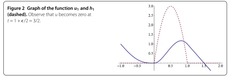
Example . Consider the problem

u(t) +u(t) +u(–t) =h(t), t∈R; u() = , (.)

where∈R,h(t) = x(–x)χ[,](x) andχ[,]is the characteristic function of the interval [,]. Observe thath is continuous. By means of the expression of the Green’s function for problem (.), we see that its unique solution is given by

u(t) = ⎧ ⎪ ⎪ ⎪ ⎪ ⎪ ⎨ ⎪ ⎪ ⎪ ⎪ ⎪ ⎩

–t–, ift< –,

–t– t, if –<t< ,

t_{– ( + }_)t_{+ }_t_, _{if  <}_t_<_,

–t+ +, ift>.

(14)

Figure 2 Graph of the functionu1andh1 (dashed).Observe thatubecomes zero at

t= 1 +/2 = 3/2.

The case (C.) is very similar,

G(t,s) = ⎧ ⎪ ⎪ ⎪ ⎪ ⎪ ⎪ ⎪ ⎪ ⎨ ⎪ ⎪ ⎪ ⎪ ⎪ ⎪ ⎪ ⎪ ⎩

 +a(t–s), ≤s≤t,

– –a(t–s), t≤s≤,

a(s+t), –t≤s≤,

–a(s+t), ≤s≤–t,

, otherwise.

Lemma . Assume a= –b.Then,if a> ,the Green’s function of problem(.)is

• positive on{(t,s), –t<s< },{(t,s),  <s<t}and{(t,s),  <s< –t}, • negative on{(t,s),t<s< }if and only ift∈(–/a, ),

and,if a> ,the Green’s function of problem(.)is

• negative on{(t,s), –t<s< },{(t,s),t<s< }and{(t,s),  <s< –t}, • positive on{(t,s),  <s<t}if and only ift∈(, –/a).

Lemma . Assume a= –b.Then we have the following:

• ifa> ,the Green’s function of problem(.)is non-negative on[, +∞)×R, • ifa< the Green’s function of problem(.)is non-positive on(–∞, ]×R,

• the Green’s function of problem(.)changes sign in any other strip not a subset of the aforementioned.

Again, for this particular case we have another way of computing the solution to the problem.

Proposition . Let a= –b,H(t) :=_th(s) ds andH(t) :=_tH(s) ds.Then problem(.) has a unique solution given by

u(t) =H(t) –H(t) – a He(t) –He(t)

+c.

Proof The equation is satisﬁed, since

u(t) +a u(t) –u(–t)=u(t) + auo(t) =h(t) – aHo(t) + aHo(t) =h(t).

(15)

Example . Consider the problem

x(t) +λ x(–t) –x(t)=λt

_{– t}₊_λ

( +t₎ , x() =λ

forλ∈R. We can apply the theory in order to get the solution

u(t) = 

 +t+λ( + λt)arctant–λ

_ln _{ +}_t₊_λ_{– ,}

whereu(t) =¯ _+_t +λ( + λt)arctant–λln( +t) – .

Observe that the real function

h(t) :=λt

_{– t}₊_λ

( +t₎

is positive onRifλ>  and negative onRfor allλ< –. Therefore, Lemma . guarantees thatu¯will be positive on (,∞) forλ>  and in (–∞, ) whenλ< –.

Competing interests

The authors declare that they have no competing interests. Authors’ contributions

All authors contributed equally to the writing of this paper. All authors read and approved the ﬁnal manuscript. Acknowledgements

The authors are thankful to the anonymous referees for the careful reading of the manuscript and suggestions. This work was supported in part by FEDER and Ministerio de Educación y Ciencia, Spain, project MTM2010-15314. The second author was supported by FPU scholarship, Ministerio de Educación, Cultura y Deporte, Spain.

Received: 23 December 2013 Accepted: 8 April 2014 Published:07 May 2014

References

1. Silberstein, L: Solution of the equationf(x) =f(1/x). Philos. Mag.7(30), 185-186 (1940)

2. Wiener, J, Watkins, W: A glimpse into the wonderland of involutions. Mo. J. Math. Sci.14(3), 175-185 (2002) 3. Piao, D: Pseudo almost periodic solutions for diﬀerential equations involving reﬂection of the argument. J. Korean

Math. Soc.41(4), 747-754 (2004)

4. Piao, D: Periodic and almost periodic solutions for diﬀerential equations with reﬂection of the argument. Nonlinear Anal.57(4), 633-637 (2004)

5. Kuller, RG: On the differential equationf=f◦g, whereg◦g=I. Math. Mag.42, 195-200 (1969) 6. Shah, SM, Wiener, J: Reducible functional-differential equations. Int. J. Math. Math. Sci.8, 1-27 (1985) 7. Watkins, W: Modified Wiener equations. Int. J. Math. Math. Sci.27(6), 347-356 (2001)

8. Wiener, J: Generalized Solutions of Functional-Differential Equations. World Scientific, River Edge, NJ (1993) 9. Watkins, W: Asymptotic properties of differential equations with involutions. Int. J. Pure Appl. Math.44(4), 485-492

(2008)

10. Aftabizadeh, AR, Huang, YK, Wiener, J: Bounded solutions for diﬀerential equations with reﬂection of the argument. J. Math. Anal. Appl.135, 31-37 (1988)

11. Gupta, CP: Existence and uniqueness theorems for boundary value problems involving reﬂection of the argument. Nonlinear Anal.11(9), 1075-1083 (1987)

12. Gupta, CP: Two-point boundary value problems involving reﬂection of the argument. Int. J. Math. Math. Sci.10(2), 361-371 (1987)

13. O’Regan, D, Zima, M: Leggett-Williams norm-type ﬁxed point theorems for multivalued mappings. Appl. Math. Comput.187(2), 1238-1249 (2007)

14. O’Regan, D: Existence results for diﬀerential equations with reﬂection of the argument. J. Aust. Math. Soc. A57(2), 237-260 (1994)

15. Andrade, D, Ma, TF: Numerical solutions for a nonlocal equation with reﬂection of the argument. Neural Parallel Sci. Comput.10, 227-233 (2002)

16. Ma, TF, Miranda, ES, de Souza Cortes, MB: A nonlinear diﬀerential equation involving reﬂection of the argument. Arch. Math.40(1), 63-68 (2004)

17. Wiener, J, Aftabizadeh, AR: Boundary value problems for diﬀerential equations with reﬂection of the argument. Int. J. Math. Math. Sci.8(1), 151-163 (1985)

(16)

19. Cabada, A, Infante, G, Tojo, FAF: Nontrivial solutions of perturbed Hammerstein integral equations with reﬂections. Bound. Value Probl.2013, 86 (2013)

20. Azbelev, NV, Domoshnitsky, A: A question concerning linear diﬀerential inequalities - I. Diﬀer. Uravn. (Minsk)27, 257-263 (1991)

21. Azbelev, NV, Domoshnitsky, A: A question concerning linear diﬀerential inequalities - II. Diﬀer. Uravn. (Minsk)27, 641-647 (1991)

22. Agarwal, RP, Berezansky, L, Braverman, E, Domoshnitsky, A: Nonoscillation Theory of Functional Diﬀerential Equations with Applications. Springer, New York (2012)

23. Domoshnitsky, A: Maximum principles and nonoscillation intervals for ﬁrst order Volterra functional diﬀerential equations. Dyn. Contin. Discrete Impuls. Syst., Ser. A Math. Anal.15, 769-814 (2008)

24. Domoshnitsky, A: Nonoscillation interval forn-th order functional diﬀerential equations. Nonlinear Anal., Theory Methods Appl.71, e2449-e32456 (2009)

25. Domoshnitsky, A, Maghakyan, A, Shklyar, R: Maximum principles and boundary value problems for ﬁrst-order neutral functional diﬀerential equations. J. Inequal. Appl.2009, Article ID 141959 (2009)

10.1186/1687-2770-2014-99