http://www.sciencepublishinggroup.com/j/jbed doi: 10.11648/j.jbed.20170204.13
Dynamic Relationship Between Fiscal Policy and Economic
Growth in Nigeria (Long and Short Run Analysis)
Paul Ndubuisi
Department of Banking and Finance, Abia State University, Okigwe, Uturu
Email address:
pauloabsu2017@gmail.com
To cite this article:
Paul Ndubuisi. Dynamic Relationship Between Fiscal Policy and Economic Growth in Nigeria (Long and Short Run Analysis). Journal of Business and Economic Development. Vol. 2, No. 4, 2017, pp. 215-226. doi: 10.11648/j.jbed.20170204.13
Received: May 9, 2017; Accepted: May 20, 2017; Published: July 20, 2017
Abstract:
This study investigates empirically the fiscal policy impact on the economic growth index in Nigeria for the period 1985-2015. Data for the study were collected from secondary sources. The expost facto research design was adopted for the study. The data were analysed using OLS multiple regression, unit root test, co-integration and Error Correction mechanism (ECM). The results revealed that the variables were all stationary at level and co-integrated of the same order in the long-run. The result also showed that fiscal policy significantly influenced the rate of growth in Nigeria economy. It was therefore recommended that government should ensure transparency in budget implementation and fiscal discipline to put Nigeria on the path of sustainable growth.Keywords:
Fiscal Policy, Economic Growth, Capital Expenditure, Recurrent Expenditure, Domestic Debt1. Introduction
The Nigerian economy has been plagued with several challenges over the years. Researchers have identified some
of these challenges as: gross mismanagement /
misappropriation of public funds, corruption and ineffective economic policies, lack of integration of macroeconomic plans and the absence of harmonization and coordination of fiscal policies as well as inappropriate and ineffective policies. Imprudent public spending and weak sectorial linkages and other socioeconomic maladies constitute the bane of rapid economic growth and development.
Fiscal Policy is the budgetary policy of the government relating to revenue (taxes), public expenditure, public borrowing and deficit financing Sanni, [1]. Thus, fiscal policy aims at stabilizing the economy. As noted by Anyanwu [2], the objective of fiscal policy is to promote economic conditions conducive to business growth while ensuring that any such government actions are consistent with economic stability.
Economic Growth on the other hand is an increase in real output or real per capita output of an economy Udabah, [3]. Similarly, Kuznets [4] also defined economic growth as a long term rise in capacity to sustain increasingly, diverse economic goods and services to its population, growing
capacity based on advancing technology, institutional and ideological adjustments that it demands. The interpretation of economic growth emphasizes a "sustained" rise in the output level which is the only manifestation of economic growth.
However, some scholars did not support the claim that increasing fiscal policy promotes economic growth, instead they assert that higher government expenditure may slowdown overall performance of the economy. For instance, in an attempt to finance rising expenditure, government may increase taxes and/or borrowing. Higher income tax discourages individual from working for long hours or even searching for jobs. This in turn reduces income and aggregate demand. In the same vein, higher profit tax tends to increase production costs and reduce investment expenditure as well as profitability of firms. Moreover, if government increases borrowing (especially from the banks) in order to finance its expenditure, it will compete (crowds-out) away the private sector, thus reducing private investment.
expenditure to GNP has been rising and corresponds with the rising share hypothesis. About 60 percent of the population lives on less than US$1 per day. This is inspite of astronomical increases in government expenditure over the years. It is on this background that this study would investigate the impact of fiscal policy on the economic growth of Nigeria.
1.1. Statement of the Problem
The relationship between fiscal policy and economic growth has continued to generate series of debate among scholars. Government performs two functions protection (security) and provisions of certain public goods Abdullah, [7] and Al-Yousif, [8]. Protection function consists of the creation of rule of law and enforcement of property rights. This helps to minimize risks of criminality, protect life and property, and the nation from external aggression. Under the provisions of public goods are defense, roads, education, health, and power, to mention a few. Some scholars argue that increase in government expenditure on socio-economic and physical infrastructures encourages economic growth. For example, government expenditure on health and education raises the productivity of labour and increase the growth of national output. Similarly, expenditure on infrastructure such as roads, communications, power, reduces production costs, increases private sector investment and profitability of firms, thus fostering economic growth. Supporting this view, scholars such as Al-Yousif, [8], Abdullah, [7], Ranjan and Sharma,[9] and Cooray, [10] concluded that expansion of government expenditure contributes positively to economic growth.
For instance Ram [11] found that a stronger positive relationship exists between fiscal policy and economic growth in lower income countries than in higher income countries. In contrast, Landau [12] concluded that the data he examined support the view that government spending is associated with a reduction in a country's capacity to grow. Easterly [13] seems to support Landau's results as he implied that government consumption spending is negatively associated with economic growth and GDP per capita. Ezirim and Muoghalu [14] investigated the extent to which factors like population growth, urbanization effects and taxation affect the size of public expenditure in less developed countries like Nigeria; and concluded that inflation constituted the most important factor that accounted for changes in government financial management. Offurum [15] in an extensive study investigated the impact of public expenditure on economic growth.
There exists a consensus in the literature that an adequate and effective macroeconomic policy is critical to any successful development process aimed at achieving high employment, sustainable economic growth, price stability, long-term viability of the balance of payments and external equilibrium. The poor growth performance of the Nigerian economy since 1986 has generated interest in issue of growth and development. From 1970 to 1985 there was financial repression. However, financial liberalization was introduced
in 1986 to realise necessary finance to promote growth. This has made it necessary to study and understand the relationship between finance and growth. Nigeria is endowed with enormous potential for growth and development with her vast oil and gas resources, rich and expensive agricultural land, solid minerals and abundant human resources. Despite these factors, since 1960 when she got her independence from Britain, the successive governments have not done enough to put the nation's resources to effective productive use as to chart the path of growth and development. The net result is that the Nigerian economy is now performing below her potential as the "crown prince of the Gulf of Guinea".
Prior to 1975, there were lots of uncontrolled spending in the economy. The monetary control was minimal in the domestic science, ports were congested, the civil service was overloaded and largely corrupt and the economy lacked positive thrust. Despite the lofty place of fiscal policy in the management of the economy, the Nigerian economy is yet to come on the path of sound growth and development. Studies by Agiobenebo [16], Gbosi [17] and Okowa [18] indicate that the economy is still marred by chronic unemployment, rising rate of inflation, dependence on foreign technology, monoculture foreign exchange earnings from crude oil, and more. Furthermore, stagnating revenue mobilization in particular and some upward movements in expenditures led to a reversal of the fiscal stabilization process since the second half of the Nineties. An improved fiscal performance during 2003-04 engendered by containment of non-planned expenditures and supported by high revenue mobilization on the back of buoyant real activity paved the way for renewed commitment towards fiscal consolidation in Nigeria. Arising from the issue above, this paper seeks to examine the impact of fiscal policy on economic growth in Nigeria and thus fill the gap in literature.
1.2. Theoretical Literature
Literatures abound on the relative effectiveness of fiscal policy in developed and developing countries of the world. The literature of fiscal policy provides guidance on how expenditure assignment could be optimally designed on the grounds of allocating efficiency, manageability, autonomy and accountability. Overtime, the role of government in an economy has continued to increase in absolute and relative terms for the past decades, this rising role had led the postulation of some economic theories that concerns the fiscal policy and the growth of the economy by some scholars in economics. Theoretically, it is argued that total government expenditure adjusts more rapidly than revenue to price level variation in such a way that bank-financed budgetary deficit set in (Aghevli and Khan, [19]). The following theories discusses fiscal policy and economic growth
1.2.1. The Keynesian Hypothesis
became clear that the market economy can no longer check economic depression that was not foreseen in the periods of the classical economists.
Keynes therefore argued, that the deficiencies that surround demand and the subsequent decline in production and employment could be eliminated through government intervention. This can be done by way of government expenditures on public works that will stimulate the economy to further activities through the multiplier and the accelerator. This new turn in economic event by Keynes formed the new era in economic thinking and policies. The use of fiscal policy therefore, brought into focus the government's active participation in the regulation and manipulation of aggregate economic activities. To this effect, Keynes believed that changes in saving and investment are responsible for changes in business activity and employment in an economy. He therefore, advocated for the use of fiscal policy by the government through deficit financing to tackle economic depression.
Since 1939, the most popular method of controlling business fluctuations or maintaining economic stability had been the deliberate use of fiscal policy. To Keynes, the fiscal policy of the Government involving taxation, debt and expenditure has to be anti-cyclical in behaviour. The Government will therefore spend more of its income during the period of depression and less in prosperity through fiscal policy. The intended objective is to ensure economic stability. In both developed and developing countries, the Government has a vital role to play in stimulating business activities. This objective can be achieved by using fiscal policy. It is designed to ensure adequate stabilization of income and employment levels of the economy, distribution of justice and optimum allocation of productive resources. It also aims at bringing about a reduction in inequalities in income and wealth.
1.2.2. Wagner's Law of Increasing State Activity
Wagner [20] was a German political economist who based his law on increasing state activities and historical facts, primarily in Germany. He studied the German economy overtime and observed a correlation growth between national
output andthe public expenditure in the economy.
He expressed the view that there was an inherent tendency for the activities of different layers of government (such as central and state governments) to increase both intensively and extensively. That is, there is a functional relationship between the growth of an economy and the growth of government activities, so that the government sector grows faster than the economy.
Wagner expressed the view that public expenditure increase at a faster rate than the national output. That is, the share of public sector in the economy will increase as the economy growth proceeds. Wagner argued that a functional cause and effect relationship exist between the growth of an industrializing economies. This long term hypothesis has it that social progress was the basic cause of the relative growth of the government in industrializing economies. The chain
reaction circumstances are that social progress leads to a growth of government functions, which in turn, leads to the absolute and relative growth of economic activity.
1.3. Empirical Literature
The impact of fiscal policy on economic growth has generated large volume of empirical studies by various scholars in economic literature with mixed findings using cross sectional, time series and panel data. Fiscal policy is generally believed to be associated with growth, or more precisely, it is held that appropriate fiscal measures in particular circumstances can be used to stimulate economic growth and development (Khosravi and Karimi, [21]). Hence, this section of the study seeks to review relevant empirical studies that have examined the impacts of fiscal policy in the actualization of sustainable growth and development.
Differing opinions have indeed continued to emerge on how fiscal policy can affect economic activities. The genesis of these controversies has been traced to the theoretical exposition of the different schools of thought namely; the classical, the Keynesian, and the Neoclassical school of thought (Tchokote, [22]).
To the classical school of thought, fiscal deficits incessantly financed by debt crowds-out private investment and by extension, lowering the level of economic growth. As summarized by Tchokote [22]), the classical economists believe that debt issued by the public has no effect on the private sector savings. To them, a deficit financed by increasing the supply of securities, ceteris paribus reduces its price and raises real interest rates and this crowds out private investment. In sum, excessive deficit can lead to poor economic performance.
In contrast, the Keynesian school of thought postulates a positive relationship between deficit financing and investment and consequently on economic growth. This school of thought sees fiscal policy as a tool of overcoming fluctuations in the economy. The school also regards deficits financing as an important tool to achieve a level of aggregate demand consistent with full employment. They asserted that when debt is used to finance government expenditures, consumers' income will be increased and given that resources are not fully utilized, crowding-out of private investment by high interest rates would not occur.
The position of the Keynesian school of thought on the possible effects of fiscal deficits on economic activities were challenged by the Neoclassical school of thought on the premise that the former school ignored the significance of how fiscal deficits are financed on the effect of this policy variable on macroeconomic performance. The Neoclassical school postulates that the manner in which deficits are financed is capable of influencing the level of consumption and investment and by extension affect economic growth.
increase, consumers save rather than spend the income from tax cut. If the Ricardian equivalence holds, therefore, the reduction of fiscal deficit will not affect the level of consumption or balance of payments in the economy and the basis for deficit reduction, as part of stabilization programmes, no longer exist.
In addition to the controversies among the different schools of thought on the possible linkage between fiscal policy and economic growth, efforts have also been made by researchers to authenticate or refute the arguments of these prominent schools of thought.
Therefore, the attempt to empirically test the efficacy of fiscal policy in an economy dates back to the pioneering studies of Friedman and Meiselman [23] who empirically investigated the responsiveness of general price level on economic activity represented by aggregate consumption to change in money supply and autonomous government expenditure using ordinary simple linear regression model to estimate the US data from 1897-1957. In their conclusion, they found out that a stable and predictable causal relationship existed between demand and money supply while no such significant relationship was observed for government expenditure (Bogunjoko, [24]). Hence, there was a stable aggregate and money supply for the period.
Babalola and Aminu [25] investigated the impact of fiscal policy on economic growth in Nigeria over the period of 1977-2009. Unit roots of the series were examined using the Augmented Dickey - Fuller technique after which the co-integration test was conducted using the Engle - Granger Approach. Error correction models were estimated to take care of short-run dynamics. The overall results indicated that productive expenditure positively impacted on economic growth during the period of coverage and a long-run relationship exists between them as confirmed by the co-integration test.
Philips [26] critically analyzed the Nigerian fiscal policy between 1960 and 1997 with a view to suggesting workable ways for the effective implementation of vision 2010. He observed that budget deficit have been an abiding feature in Nigeria for decades. He noted that except for the period 1971 to 1974, and 1979, there has been an overall deficit in the federal government budgets each year since 1960 to date. The chronic budget deficits and their financing largely by borrowing, he asserts, have resulted in excessive money supply, worsened inflationary pressures, and complicated macroeconomic instability, resulting in negative impact on external balance, investment, employment and growth. He however, contends that fiscal policy will be an effective tool for moving Nigeria towards the desired state in 2010 only if it is substantially cured of the chronic budget deficit syndrome it has suffered for decades.
Loto [27] investigated the growth effects of government expenditure in Nigeria over the period of 1980 to 2008, with a particular focus on sectorial expenditures. Five key sectors were chosen (security, health, education, transportation, communication and agriculture). A linear ordinary least square (OLS) regression analysis was done. The variables
were tested for stationarity and co-integration analysis was also carried out using the Johansen co-integration technique. Also error correction test was performed. The result showed that in the short-run, expenditures on education and agriculture were found to be relatively related to economic growth. While the impact of education was not significant, that of agriculture was found to be significant. Expenditure
on health, national security, transportation and
communication were found to be positively related to economic growth. The result of that of health was significant while that of national security, transportation and communication were found to be insignificant. Loto opined that it is possible that in the long run expenditure on
education could be positive if brainis checked,
Egwaikhide [28] appraised the implication of Nigeria budget deficit profile for inflation and the current account balance. Evidence indicates that fiscal indiscipline in terms of lack of control over expenditure is the major determinant of budget deficit in Nigeria. While its mode of financing has aggravated inflation in the country, most importantly, it revealed that budget deficit correlates highly with current account deficit, implying that external disequilibrium is partly attributable to endogenous factors.
Akpan [29] used a disaggregated approach to determine
the components (that include capital, recurrent,
administrative, economic services, social and community service and transfers) of government expenditure that enhances growth and those that do not. The author concluded that there was no significant association between most components of government expenditure and economic growth in Nigeria.
However, in his study, showed that the major cause of macroeconomic instability and low growth in national output were the in unsustainable level of fiscal deficits, financed through borrowing from the banking system and poor management of deficit finance which gave little attention to the heavy scheduled debt service obligations. He highlighted that a prudent fiscal policy can contribute to the achievement of macroeconomic stability and growth. However, deficit financing by borrowing from the banking system and poor management of deficit finance can also lead to instability and poor economic performance.
Koman and Bratimasrene [30], studies the economy of Thailand, they made use of the Granger causality tests. Their findings were that government expenditures and economic growth are not co-integrated but indicated a one-dimensional relationship. This is because causality runs from government expenditure to growth; also their results indicated a significant positive effect of the government spending on economic growth.
Daniel and Adams [32] employed the autoregressive distributed lag bounds testing approach to co-integration to investigate the extent to which democracy and government spending have had an impact on economic growth in Ghana over the period 1960-2008. The empirical results reveal a support of high efficiency of government spending in democracies hypothesis. The results also show that democracy and government spending go hand in hand to have a positive impact on economic growth in Ghana in both the long and short run.
Ubesie [33], in his study of the effect of fiscal policy on economic growth noted that rising capital inflow will increase economic growth. On the basis of his findings, he recommended that the government should formulate and implement viable fiscal policy options that will stabilize the economy. This could be achieved through the practice of true fiscal federalism and decentralization of levels of government in Nigeria. Again, there should be consistency in macroeconomic policies implementation in the non-oil sectors of the economy by providing incentives to foreigners (especially tax holidays) wishing to invest in the agricultural sector and manufacturing sectors.
2. Research Methodology
An ex post facto research design was adopted in this study because already existing data were used. The study mainly relied on annual time series secondary data covering the period 1985 to 2015. The information was sourced from Central Bank of Nigeria (CBN) statistical Bulletin and National Bureau of Statistics (NBS). The variables obtained include the following capital expenditure, Domestic Debt, Non-Oil Revenue, Recurrent Expenditure and Gross Domestic Product.
3. Data and Model Specification
3.1. Data
This study uses annual data covering the period from 1985 to 2015. Four component of public sector (or fiscal policy instrument) expenditure are employed: recurrent expenditure and capital expenditure, Non-oil revenue and domestic debt is included in the model. These factors have been identify among the most significant determinants and proxies for fiscal policy instrument. Table 1 provides additional information on all the variables.
Table 1. List of variables.
Variable/Apriori Definition Unit Sources
RGDPC Represents the Gross Domestic Product. It captures economic growth of Nigeria from
1985-2015. InRGDP
CBN Statistical Bulletin [38]
DD (-) It represent all local borrowing financial and non-financial institutions in Nigeria. lnDD CBN Statistical Bulletin [38]
NOILR (+) It represents all the income from dgp other than oil sector. We expect this variable to
positive in the model. CBN Statistical Bulletin [38]
CEX (+)
Represents public sector capital expenditure which includes capital expenditure on administration. economic services, social and community services, transfers etc. In consistent with Abu-Bader and Abu-Qarn [31].
CBN Statistical Bulletin [38]
REX (+) Represents public sector recurrent expenditure on administration. Economic services,
social.' and community services, transfers etc CBN Statistical Bulletin [38]
Author’s Compilation
Following the theoretical framework, the functional model for this study is presented thus:
GDP = f (CEX, DD, NOILR, REX) (1)
The above model can be transformed into econometrics model as follows
In GDP = b0 + b1In CEX + b2In DD + b3In NOILR + b4In REX + Ut (2)
Where: b1, b3, b4>0 while b2< 0
In = natural logarithms of the variables. Where;
GDP = Gross Domestic Product, CEX = Capital Expenditure, DD = Domestic Debt
NOILP = Non- oil Revenue, REX = Recurrent Expenditure
b0 = The intercept of the regression equation
b1, b2, b3, and b4 are the slope co-efficient of the
independent variables
Ut = Error term that captures the variables not explicitly
included in the model
To improve the functional form of the model, the author
followed the standard linear transformation.. Also
transforming the variables into logarithms helps to reduce the possibility of conditional heteroscedasticity in the model (Gujarati, [34]). Accordingly, a log form of the model is introduced into equation (2) and it is stated thus:
3.2. Methodlogy
The study adopted the following methods for analysis of data. These include OLS multiple regression, Unit root Test, co-integration test and Error correction Mechanism (ECM) test.
3.2.1. Unit Root Test
problem of spurious regression. The ADF unit root test was adopted because it helps to avoid the problem of spurious regression, and adjusts appropriately for the occurrence of serial correlation (Ogwuru and Ewubare, [39]). Therefore, before applying this test, the author determine the order of integration of all variables using unit root tests by testing for
null hypothesis : = 0 (i.e has a unit root), and the
alternative hypothesis is : < 0.
3.2.2. Co-integration Test
Having established the order of integration, the next thing is to use Johansen’s [35] procedure of maximum likelihood to determine the number of cointegrating vectors.
Consider the following level vector autoregression, VAR of order
= + +……..+ + (3)
Where is a ( × 1) vector of fiscal policy and growth in
log form that are integrated at order one- commonly denoted
1 (1), n=5, are the parameters to be estimated, are the
random errors. This (VAR) can be re-written as;
∆ = + ∏ + ∑&'' Γ&∆ &+ (4)
Where,
Π = ∑&' &− 1 and Γ&= − ∑*'&+ * (5)
If the coefficient matrix Π has reduced rank , < , then
there exist × , matrices of - and each with rank , such
that
Π = - . (6)
Where , is the number of co-integrating relationship, the
element is - is known as the adjustment parameters in the
vector error correction model and each column of is a
cointegrating vector. It can be shown that, for a given ,, the
maximum likelihood estimator of define the combination
of that yield the , largest canonical correlations of
∆ with after correcting for lagged differences and
deterministic variables when present. The two different likelihood ratio test of significance of these canonical correlations are the trace test and maximum eigenvalue test, shown in equation 7 and 8 respectively below
/0123(,) = −4 ∑9&'0+ ln (1 − /87) (7)
and
/:1;(,, , + 1) = −4 (1 − /=0+ ) (8)
Here, T is the sample size and /=& is the >? ordered
eigenvalue from the Π matrix in equation 3 or largest
canonical correlation. The trace tests the null hypothesis that
the number of , co-integrating vector against the alternative
hypothesis of co-integrating vector where is the number of endogenous variables. The maximum eigenvalue tests the
null hypothesis that there are , cointegrating vectors against
an alternative of , + 1 (see Brooks [36]).
3.2.3. Error Correction Mechanism (ECM)
Having determined whether or not co-integration exists, we applied the ECM to ascertain the speed of adjustment from the short-run equilibrium to the long-run equilibrium state. If co-integration is accepted, it suggests that the model is best specified in the first difference of its variables with one lag of the residual [ECM (-1)] as additional regressor. The (ECM) incorporates the variables at both side levels and
first differences and thus captures the short-run
disequilibrium situations as well as the long-run adjustments between variables (Mukhtar et al,[37]). This study uses Akaike information criteria for selected the optimal lag length. The short run equilibrium relationship is tested using vector error correction model (VECM). VECM is restricted VAR that has cointegration restriction built into the specification. The VECM analysis in this study is based on equation 2 and it involves five cointegrating vector as thus:
∆ @AB = -C+ ∑9 &∆ @AB +
&' ∑ D&∆ EFG+ ∑ H&∆ AADEFG+
9 &'C 9
&'C
∑ H&∆ DEFG+
9
&'C ∑ H&∆ DEFG+
9
&'C / IJK + (9)
IJK is the error correction term obtained from the cointegration model. The error coefficients (/ ) indicate the rate at
which the cointegration model corrects its previous period’s disequilibrium or speed of adjustment to restore the long run
equilibrium relationship. A negative and significant IJK coefficient implies that any short run movement between the
dependant and explanatory variables will converge back to the long run relationship.
4. Data Analysis and Discussion of Results
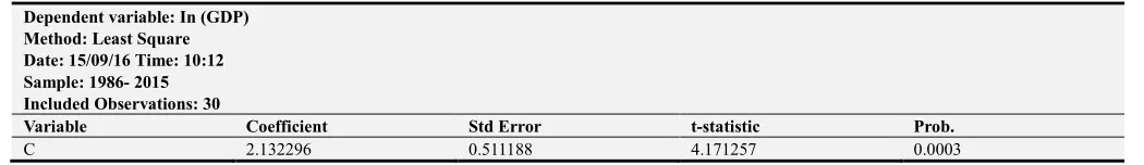
Table 2. Level Series Multiple Regression.
Dependent variable: In (GDP) Method: Least Square Date: 15/09/16 Time: 10:12 Sample: 1986- 2015 Included Observations: 30
Variable Coefficient Std Error t-statistic Prob.
Dependent variable: In (GDP) Method: Least Square Date: 15/09/16 Time: 10:12 Sample: 1986- 2015 Included Observations: 30
Variable Coefficient Std Error t-statistic Prob.
In CEX 0.035904 0.097952 0.366553 0.7170
In DD 0.574857 0.149859 3.835984 0.0008
In NOILR 0.377575 0.135785 2.780677 0.0102
In REX 0.035489 0.142877 0.248385 0.8059
R- squared 0.990086 Mean dependent var. 15.25467
Adj-R-Squared 0.988500 S.D. dep. Variable 1.934976
S.E. of Reg. 0.207501 Akaike info. crit. -0.156352
Sum sq. resid. 1.0764 1 4 Schwartz crit. 0.077181
Log. Likelihood 7.345274 Hannan-duinn crit. -0.081642
F- statistic 624.1985 Durbin Watson Stat. 1.9246
Prob. (F-statistic) 0.000000
Source: Author's Computation
Table 2 above presents the level series multiple regression-estimated model, which shows the relationship between Fiscal Policy and Economic Growth variables. From the table, In (CEX) is not significantly related to In (GDP) as well as In (REX), but In (NOILR) and In (DD) are significantly related to In GDP. The Adjusted R-squared is approximately 98.85% and the Durbin-Watson statistic is approximately, 2.0, which shows the absence of positive auto-correlation in the estimated model.
4.1. Unit Root Test
The variables were tested for unit root using the Augmented Dickey-Fuller test (ADF) at the level of first difference. The result of the unit root tests are as presented in table 3 below.
Table 3. Augmented Dickey-Fuller Unit Root Test Summary Results.
Variable ADF test Statistical
at first Difference Critical Values
Order of Integration
In CEX -5.841542
1% = -3.689194
1 (1) 5% = -2.971853
10% = -2.625121
In (DD) -4.952331
1% = -3.689194
1 (1) 5% = -2.971853
10% = -2.625121
In GDP -5.479928
1% = -3.689194
1 (1) 5% = -2.971853
10% = -2.625121
In
NOILR -7.187499
1% = -3.689194
1 (1) 5% = -2.971853
10% = -2.625121
In REX -7.655063
1% = -3.689194
1 (1) 5% = -2.971853
10% = -2.625121
Source: Author’s computation
Table 3. Augmented Dickey-Fuller Unit Root Test Summary Results.
Variable ADF test Statistical at first Difference Critical Values Order of Integration
In CEX -5.841542
1% = -3.689194
1 (1) 5% = -2.971853
10% = -2.625121
In (DD) -4.952331
1% = -3.689194
1 (1) 5% = -2.971853
10% = -2.625121
In GDP -5.479928
1% = -3.689194
1 (1) 5% = -2.971853
10% = -2.625121
In NOILR -7.187499
1% = -3.689194
1 (1) 5% = -2.971853
10% = -2.625121
In REX -7.655063
1% = -3.689194
1 (1) 5% = -2.971853
10% = -2.625121
Source: Author’s computation
Table 3 above presents the result of the ADF unit root tests. The results of the unit root tests shows that the null hypothesis of a unit root test for first difference series for all the variables can be rejected at all critical values indicating that the level series can be made stationary at the second
4.2. Co-integration Test
Applying the Johansen co-integration test, we find that the null hypothesis of no co-integration is rejected and we concluded that the variables are co-integrated in the long-run.
To determine the number of co-integrating equations, we employ the Johansen (1991) test for co-integration as shown in Table 4 below. The lag interval of 1 to 2 was used with linear deterministic test assumption.
Table 4. Johansen Co-integration Test.
Date 15/09/2016: Time: 10:30
Included observation: 27 after adjustments Sample (adjusted): 1989-2015
Series: In (GDP) In (CEX) In (DD) In (NEX) In (REX) Trend assumption: Linear deterministic trend Lag interval (in first difference): 1 to 2 Unrestricted co-integration Rank Test (Trace)
Hypothesized No of CE(s) Elgen value Trace Statistic 0.05 Critical value Prob.**
None* 0.784470 114.6544 69.81889 0.0000
At most 1* 0.751419 73.21871 47.85613 0.0000
At most 2* 0.563733 35.63511 29.79707 0.0095
At most 3 0.367219 13.23860 15.49471 0.1063
At most 4 0.032159 0.882569 3.841466 0.3475
Trace test indicates 3 co-integrating equation at 0.05 level * denotes rejection of the hyp. at 0.05 level
** Mackinnon-Haug-Michelis (1999) P-values
Unrestricted co-integration Rank Test (Max. Elgen Value)
Hypothesized no of RE(s) Elgen value Max. Eigen Statistic 0.05 Critical value Prob.**
None* 0.784470 41.43572 33.87687 0.0052
At most 1* 0.751419 37.58360 27.58434 0.0019
At most 2* 0.563733 22.39651 21.13162 0.0330
At most 3 0.367219 12.35603 14.26460 0.0980
At Most 4 0.032159 0.882569 3.841466 0.3475
Max-eigen value test indicates 3 co-integrating equation(s) at 0.05 level * denotes rejection of the hyp. at 0.05 level
** Mackinnon-Haug-Michelis (1999) P-values
Author’s computation
From the table 4 above, we can observe that the unrestricted Rank Test indicates that there are three cointegrating equations at the 5% level of significance among the dependent and independent variables. In addition the maximum Eigen value test also shows that there are three co-integrating equations at the 5% level of significance.
4.3. Error Correction Model
The existence of a long run co-integrating equilibrium provides for short-term fluctuations. Having established the existence of a long run co-integrating relationship among the variables, we therefore apply the error correction mechanism to examine the interplay of the long run and short term fluctuations in the model using the general specific approach.
Table 5. Over-parameterized Error Correction Model.
Dependent variable: D(In (GDP)} Method: Least Square
Date: 15/09/16 Time: 12:04 Sample (adjusted) 1990- 2015
Included Observations: 26 after adjustments
Variable Coefficient Std Error t-statistic Prob.
C 0.288903 0.173943 1.660909 0.1576
D(In (GDP(-1))) 0.603196 0.604738 0.997450 0.3643
D(In (GDP(-2))) -0.488351 0.599480 -0.814625 0.4523
D(In (GDP(-3))) -0.040317 0.080737 0.080737 0.9388
D(In (CEX)) 0.352873 1.276761 1.276761 0.2578
D(In (CEX(-1))) 0.635203 2.587948 2.587948 0.0490
D(In (CEX(-2))) 0.050415 0.169268 0.169268 0.8722
D(In (CEX(-3))) -0.121661 -0.612338 -0.612338 0.5671
D(In (DD) 0.088160 0.250475 0.250475 0.8122
D(In (DD(-1))) -0.252501 -0.493651 -0.493651 0.6425
D(In (DD(-2))) -0.327507 -0.901144 -0.901144 0.4088
D(In (DD(-3))) -0.244488 0.383589 -0.637370 0.5519
D(In (NOILR) 0.295864 0.242029 1.22430 0.2760
D(In (NOILR(-1))) -0.270078 0.308073 -0.876670 0.4208
Dependent variable: D(In (GDP)} Method: Least Square
Date: 15/09/16 Time: 12:04 Sample (adjusted) 1990- 2015
Included Observations: 26 after adjustments
Variable Coefficient Std Error t-statistic Prob.
D(In (NOILR(-3))) 0.150294 0.228297 0.658325 0.5394
D(In (REX) -0.196725 0.201936 -0.974192 0.3747
D(In (REX(-1))) -0.186264 0.201475 -0.924500 0.3977
D(In (REX(-2))) -0.107072 0.345784 -0.309649 0.7693
D(In (REX(-3))) -0.210860 0.550815 -0.382814 0.7176
ECM (-1) -1.468367 0.894134 -1.642223 0.1615
R- squared 0.815205 Mean dependent var. 0.223985
Adj-R-Squared 0.076025 S.D. dep. Variable 0.187079
S.E. of Reg. 0.179828 Akaike info. crit. -0.626911
Sum sq. resid. 0.161690 Schuartz crit. 0.389244
Log. Likelihood 29.14984 Hannan-duinn crit. -0.334295
F- statistic 1.102850 Durbin Watson Stat. 2.002425
Prob. (F-statistic) 0.503800
Source: Author's Computation
Table 5 above shows the over-parameterized ECM estimate with maximum lag of three. The Durbin-Watson statistic is 2.00 and Adjusted R-squared of approximately 7.6%. From the over-parameterized ECM, we obtained the parsimonious ECM as presented in table 6 below;
Table 6. Parsimonious Error Correction Model.
Dependent variable: D(In (GDP) Method: Least Square
Date: 15/09/16 Time: 12:45 Sample (adjusted) 1990-2015
Included Observations: 26 after adjustments
Variable Coefficient Std Error t-statistic Prob.
C 0.2199770 0.077402 2.839326 0.0139
D(In (GDP(-1))) 0.348640 0.186471 1.869675 0.0842
D(In (GDP(-2))) -0.598896 0.204378 -2.930333 0.0117
D(In (CEX)) 0.297643 0.112259 2.651399 0.0200
D(In (CEX(-1))) 0.544029 0.116241 4.680201 0.0004
D(In (CEX(-3))) -0.101174 0.090511 -1. 117805 0.2839
D(In (DD(-2)) -0.210844 0.174201 -1. 210353 0.2477
D(In (NOILR) 0.232511 0.082812 2.807698 0.0148
D(In (NOILR(-1))) -0.288706 0.099783 -2.893344 0.0126
D(In (NOILR(-2))) 0.118107 0.078341 1.507610 0.1556
D(In (REX) -0.195558 0.113730 -1.719502 0.1092
D(In (REX(-1))) -0.145335 0.106539 -1.364153 0.1957
ECM (-1) -0.963834 0.199139 -4.840014 0.0003
R- squared 0.793623 Mean dependent var. 0.223985
Adj-R-Squared 0.603122 S.D. dep. Variable 0.187079
S.E. of Reg. 0.117857 Akaike info. crit. 1.131840
Sum sq. resid. 0.180573 Schuartz crit. 0.502792
Log. Likelihood 27.71392 Hannan-duinn crit. 0.950697
F- statistic 4.165967 Durbin Watson Stat. 2.386429
Prob. (F-statistic) 0.008057
Author's Computation
Table 6 above presents results of the parsimonious error correction model conducted to further analyze the long run relationship between fiscal policy and economic growth and also to capture the short run deviations of the parameters from the long run equilibrium by incorporating period lagged residuals. The result shows that In (CEX) lagged three periods, is negative and not significantly related to GDP, while In (CEX) one period lag is negative and significant. In (DD) lagged two period is negative and not significant. In
run shock is approximately 96.38% per annum. The F-statistic is 4.165967 with P-value of 0.008057, which is significant. We therefore conclude that Fiscal Policies impact significantly on economic growth and reject the null
hypothesis, which states that Fiscal Policy hasno significant
impact on the economic growth of Nigeria.
4.4. Discussion of Findings
The result of this study is in line with Babalola and Aminu (2011), Loto (2011), lkem (2011), Chih-Hil (2008) and others, who observed that Fiscal policies usually have impact
on the Economy. From the above result, the Adjusted R2 that
is the coefficient of determination showed that 60.3% of the total variation in GDP is explained by the independent variables included in the model. Collectively, there is a trend between the variables, which implies that an increase in the fiscal policy variables will increase economic growth while decrease will also decrease economic growth. The P-value of the F-statistic is 0.008057, which is sufficiently low, and we conclude that there is a long run equilibrium relationship between fiscal policy and economic growth in Nigeria.
5. Summary of Findings, Conclusion and
Recommendations
The integration test revealed that there is a co-integration relationship between Fiscal Policy variables and Economic growth variable (GDP).
The findings of the study reveal that:
a. The regression result as analyzed, confirms that there
exists positive relationship between the Fiscal Policies and Economic Growth of Nigeria.
b.The relationship is statistically significant. This in
essence means that the impact of the Fiscal Policy on the Economic Growth of Nigeria is strong and
significant.
5.1. Conclusion
The study reveals that Fiscal Policies impact on the Economic Growth of Nigeria via the Gross Domestic Product (GDP). Hence the fiscal policies in every economy have the power to influence or impact the growth of that economy. Government is therefore advised to put up measures to stem up the implementation of fiscal policies as this will help in the growth of the economy.
5.2. Policy Recommendations
In the light of the research findings, the following recommendations are presented:
a. To ensure macroeconomic stability and put the Nigeria
economy along the path of sustainable growth, Government must put a stop to diversion of foreign borrowing, to unproductive use.
b.Government must curtail wasteful spending.
c. Government must embark upon specific fiscal policies
aimed at achieving increased and sustained productivity in all sectors of the economy.
d.There should be emphasis on non-oil revenue. The
system of assessment and collection of such revenue, particularly income tax, must be as simple as possible with a few taxes and uncomplicated Legislations aimed at lowering the costs of doing business in Nigeria.
e. The country should equally concentrate more on capital
expenditure and reduce allocation to recurrent expenditure. There should be expansive development of infrastructure, as it will impact on economic growth.
f. It is recommended that government should formulate
and implement viable fiscal policy options that will stabilize the economy.
Appendix
Year Capital Exp. (Nm) Domestic Debt (N million) Non-oil revenue (N million) Recurrent Expenditure
(N million) GDP (Nm)
1985 5464.700 134585.6 4126.70 7576.40 60168
1986 8526.800 134603.3 4488.50 7696.90 69147
1987 6372.500 193126.2 6353.60 15646.20 105222
1988 8340.100 263294.5 7765.00 19409.40 539085
1989 15034.10 382261.5 14739.90 25994.20 516797
1990 24048.60 472648.7 26215.30 36219.60 155506
1991 28340.90 545672.4 18325.20 38243.50 312139
1992 39763.30 875342.5 26375.10 53034.10 532613
1993 54501.80 1089680 30667.00 136727.10 683869
1994 70918.30 1399703 41718.40 89974.90 599863
1995 121138.30 2907358 135439.70 127629.80 1933211
1996 212926.30 4032300 114814.00 124491.30 2702719
1997 269651.70 4189250 166000.00 158563.50 2801972
1998 309015.60 3989450 139297.60 178097.80 2708430
1999 498027.60 4679212 224765.40 449662.40 3194015
2000 239450.90 6713575 314483.90 461600.00 4582127
2001 438696.50 6895198 903462.30 579300.00 4725086
2002 321378.10 7795758 500986.30 696800.00 6912381
2003 241688.30 9913518 500815.30 984268.10 8487031
Year Capital Exp. (Nm) Domestic Debt (N million) Non-oil revenue (N million) Recurrent Expenditure
(N million) GDP (Nm)
2005 519470.00 14610881 785100.00 1223730.00 1457223
2006 552385.80 18564595 677500.00 1390201.90 18564594
2007 759281.20 20657318 1200800.00 1589300.00 20657317
2008 960890.10 24296329 1336000.00 2117362.00 24296329
2009 1152800.00 24794239 1652700.00 2127971.50 24310724
2010 883870.00 33984754 1907600.00 3109378.51 24712669
2011 918500.00 37409861 2237900.00 3314513.33 54204800
2012 874800.00 40544100 2628771.39 3325178.00 71186530
2013 1108390.00 80092560 2950560.00 3689060.00 802222130
2014 783120.00 89043620 3275120.00 3417580.00 84312140
2015 8421000 9204340 3995154.00 3891400.00 942,66741
Source: CBN Statistical Bulletin and NBS various issues.
References
[1] Sanni (2012). Public expenditure and economic growth. African journal of economic policy 1 (1). Nigeria, university of Ibadan press.
[2] Anyanwu, J. C. (1993). Monetary economics theory: policy and institutions. Onitsha hybrid publishers ltd.
[3] Udabah. S. I (1999). An introduction to Nigerian public finance, Nigeria: linco press.
[4] Kuznets S. (1973). Modern economic growth: findings and reflections. The American economic review, 63, 3.
[5] Diamond, J. (1990). Fiscal indicators for economic growth, an illusory search. IMF working paper No 104.
[6] Longe, J, B. (1984). The Growth and Structure of Federal Government Expenditure in Nigeria. The Journal of Economics and Social Studies, 26 (1).
[7] Abdullah, H. A. (2000). The relationship between fiscal policy and Economic Growth in Saudi Arabia. Journal of Administrative Science. 12 (2).
[8] Al-Yousif, Y. (2000). Does government expenditure inhibit or promote economic growth: some empirical evidence from Saudi Arabia. Indian economic journal. 48 (2).
[9] Ranjan, K. D. & Sharma, C. (2008). Government expenditure and economic Growth, evidence from India. The lafia University journal of public finance. 6 (3).
[10] Cooray, A. (2009). Government expenditure, governance and economic growth, comparative economic studies. 51 (3). [11] Ram, R. (1986). Government size and economic growth: a
new framework and some evidence from cross-section and times-series data, American economic review. 76.
[12] Landau, D. (1983), Government expenditure and economic growth, across-country study. Southern economic journal. 12 (1).
[13] Easterly. (1992). fiscal policy and economic growth: an empirical investigation, Journal of monetary economics. 23 (3).
[14] Ezirim, B. C & Muoghalu M. I (2006). Explaining the size of public expenditure in less developed countries. Theory and empirical evidence from Nigeria. ABSU journal of management sciences, 2, (2), 134 -154.
[15] Offurum, O. (2005). Public expenditure and economic growth, African journal of economic policy. Ibadan (Nigeria), university of Ibadan press.
[16] Agiobenebo, T. J. (2003). Public sector economics: principles, theories, issues and applications. Port Harcourt: Lima Computers.
[17] Gbosi, A. N. (2002). Contemporary macroeconomic problems and stabilization policies. Port Harcourt, automatic ventures.
[18] Okowa. W. J. (1997). Oil, Systemic Corruption, Abdulistic Capitalism and Nigerian Development: A political economy Port Harcourt: paragraphics publishers.
[19] Aghevli, B. B. and M. S. Khan (1970). Inflationary and economic growth Journal of political Economy, 23 (2). [20] Wagner, A. f (1911). Staat In national ökonomischer hinsicht,
in handwörterbuch der staats wissenchaften, third edition book VII. Jena: lexis 743-745.
[21] Khosravi. A & Karimi M. S. (2010). To investigate the relationship between monetary, fiscal policy and economic growth in Iran: autoregressive distributed lag approach to cointegration. American journal of applied sciences, 7, 3. [22] Tchokote, J. (2001). Macroeconomics of fiscal deficits in
Cameroon, being a Ph.D thesis proposal presented to the department of economics, university of Ibadan Nigeria. [23] Friedman M. & Meiselman. D. (1963). The relative stability
of monetary velocity and the investment multiplier in the United States, 1897 - 1958, in commission on money and credit: stabilization policies. Englewood Cliffs, NJ: prentice Hall 165-268.
[24] Bogunjoko J. O (1997). Monetary dimensions of the Nigerian economic crisis, empirical evidence from a cointegration paradigm. The Nigerian journal of economic and social studies, 39 (2): 140-147.
[25] Babalola S. J & Aminu U. (2011). Fiscal policy and economic growth relationship in Nigeria, international journal of management and social sciences.
[26] Philips, A. O. (1997). Fiscal relations among the various tiers of government in Nigeria, journal of monetary economics. 1 (152).
[28] Egwaike, F. O (1998). Budget deficit and macroeconomic management in Nigeria, in post- structural adjustment programme. The Nigerian journal of economic and social studies, 38 (1), 3.
[29] Akpan, N. I. (2005). Expenditure, government and economic growth in Nigeria: a disaggregated approach, CBN economic and financial review.
[30] Koman, J. & Brahmasrene, T. (2007). The relationship between government expenditures and economic growth in Thailand, journal of economics and economic education research 23 (2).
[31] Abu-Bader, S. and Abu-Qarn A. S. (2003). Government expenditures, military spending and economic growth: causality evidence from Egypt, Israel, and Syria. Journal of Policy Modeling. 13 (4).
[32] Daniel S. and Samuel A. (2012). Democracy, government spending and economic growth: a case of Ghana, 1960 - 2008. The journal of applied economic research.
[33] Ubesie, M. C (2016). Effect of fiscal policy on economic growth in Nigeria journal of finance and accounting, 4, 3. [34] Gujarati, D. (2004). Basic Econometrics. United States
Military Academy, West Point.
[35] Johansen, S. (1992). Cointegration in partial systems and the efficiency of single-equation analysis. Journal of econometrics, 52 (3), 389-402.
[36] Brooks, C. (2014). Introductory econometrics for finance. Cambridge university press.
[37] Mukhtar T, M. Z., & Ahmed, M. (2007). An empirical investigation for twin deficits hypothesis in Pakistan, journal of economic corporation, 28 (4), 63 - 80.
[38] Central Bank of Nigeria (CBN) Bulletin 2015.