Numerical solution of nonlinear SPDEs using a multi-scale method
Mahmoud Mohammadi Roozbahani
Faculty of Mathematical Sciences, University of Guilan, P. O. Box 19141–41938, Rasht, Iran.
E-mail: [email protected]
Hossein Aminikhah∗
Faculty of Mathematical Sciences, University of Guilan, P. O. Box 19141–41938, Rasht, Iran.
E-mail: [email protected]
Mahdieh Tahmasebi
Faculty of Mathematical Sciences, Tarbiat Modares University, P. O. Box 14115–134, Tehran, Iran.
E-mail: [email protected]
Abstract In this paper we establish a new numerical method for solving a class of stochastic partial differential equations (SPDEs) based on B-splines wavelets. The method combines implicit collocation with the multi-scale method. Using the multi-scale method, SPDEs can be solved on a given subdomain with more accuracy and lower computational cost than the rest of the domain. The stability and consistency of the method are provided. Also numerical experiments illustrate the behavior of the proposed method.
Keywords. Multi-scale method, Cubic B-splines, Stochastic partial differential equations.
2010 Mathematics Subject Classification. 60H35, 65D07, 65T60.
1. Introduction
Many interesting problems in physics, science, engineering and finance can be modeled using stochastic partial differential equations (SPDEs). Numerical meth-ods for evolution SPDEs have been studied extensively over the past two decades [1, 7, 9, 11-14, 17, 18, 32, 41-46]. In recent years, numerous works have been focusing on the development of more advanced and efficient methods for SPDEs such as fi-nite element methods [1, 4, 8-10, 19, 22, 24, 26, 42, 46], fifi-nite difference methods [13,15, 31,35,36, 38,39, 41,43], spectral Galerkin methods [11, 18, 20, 21, 23, 28, 29, 32-34] and also some numerical methods that are based on the wavelet approx-imations [9, 16, 18, 25, 27, 40]. In this work, we intend to extend the multi-scale
Received: 1 May 2017 ; Accepted: 10 March 2018.
∗Corresponding author.
method [2,3,30] to approximate the solutions of the following SPDEs,
du(x, t) = (Au(x, t) +f(u(x, t)))dt+g(u(x, t))dW(t), (1.1)
u(x,0) =h(x), u(0, t) =u(m, t) = 0,
by wavelets where A ≡ ∂x∂22, f is Lipshcitz function, g is a function with bounded derivative and ˙W(t) is a time white noise. The existence of strong solutions of this SPDE have been investigated in [44]. We are interested in applying the multi-scale method to equation (1.1) to approximate the solution based on the wavelet expansion. In this method, first we reshape wavelets in such a way that satistify the boundary conditions exactly, second, the implicit θ-Euler-Maruyama method is employed to discretize time. Then we approximate the operators in matrix forms to obtain a sys-tem, which due to the multi-scale method will divide to two smaller systems with less computations. Finally, we combine the solutions of these systems to approximate the solution of equation (1.1). This method is suitable to approximate the solutions of sto-chastic equations because in every realization of the approximation less computation should be done.
The outline of the paper is as follows. In section2, the Multi-resolution analysis and the operational matrices of wavelets are explained and we introduce main notation used throughout the paper. In section3, we propose our stochastic the multi-scale method based on the wavelets. In section4, consistency and stability criterions of the method are investigated. In the last section, numerical simulations are presented to illustrate the efficiency of the method.
2. Preliminary remarks
In this section we use the multi-resolution analysis (MRA), to represent derivatives of functions in matrix-form on a given subdomain, with respect to cubic b-splines. From [5], we know that MRA is a sequance of subspaces Vj in L2(R), which satisfy
the following properties: (i) Vj ⊂Vj−1, j∈Z,
(ii) ∪
j∈ZVj is dense inL2(R) andj∩∈ZVj={0}, (iii) Iff(·)∈V0thenf
(
2−j·)∈Vj and vice versa, (iv) ϕ(· −k), k∈Zis a Riesz basis ofV0.
It can be inferred that the family
{
ϕj,k(x) = 2−
j
2ϕ(2−jx−k), k∈Z
} ,
is a basis for Vj. One may construct wavelets by completing the spaces Vj to the spaceVj−1 by means of a spaceWj , i.e. Vj−1 =Vj⊕Wj, in such a way that there exists a functionψ such that Wj is spanned by ψ(2−j.−k). For each j ∈ Z, the space Wj serves as the orthogonal complement of Vj in Vj−1. In the biorthogonal
case [6], the spaceWj is orthogonal to the dual ofVj. The sequence
{ e Vj
}
biorthogonal wavelets if each of the sets {ψjk: j, k ∈Z} and
{ e
ψjk: j, k ∈Z
}
are Riesz basis ofL2(R) and they are biorthogonal to each other in the following sense
⟨ψjk,ψeim⟩=δj, iδk, m ∀j, k, l, m ∈Z,
where⟨. , .⟩is the inner product onL2(R) andδi, jis Kroneker delta function. Design-ing biorthogonal wavelets allows more degrees of freedom than orthogonal wavelets. One additional degree of freedom is the possibility to construct symmetric wavelet functions. Since they define a multi-resolution analysis, the dual functions must sat-isfy,
e
ϕ=∑
k
ehkϕe(2x−k) and ψe=
∑
k
e
gkϕe(2x−k), (2.1)
whereehk andegk have been introduced in [5]. The B-splines which are symmetric and have finite support, are defined by the following recursively formula
B0= 1[0,1),
Bk+1(x) =21k
k∑+1
i=0 (
k+ 1
i )
Bk(2x−i).
(2.2)
Furthermore, we have
d
dxBi+1(x) =Bi(x)−Bi(x+ 1), (2.3) d2
dx2Bi+1(x) =Bi−1(x)−2Bi−1(x+ 1) +Bi−1(x+ 2). (2.4)
In this work, we consider the cubic B-splines,
ϕ(x) =B3(x) =
1 6
4 ∑
i=0 (
4
i )
(−1)i(x−i)3+, (2.5)
where
xk+=
{
xk, x >0, 0, x≤0.
The cubic B-spline wavelet is given by
ψ(x) = 1 27
(
5ϕ(2x+ 5) + 20ϕ(2x+ 4) +ϕ(2x+ 3) −96ϕ(2x+ 2)−70ϕ(2x+ 1) + 280ϕ(2x) −70ϕ(2x−1)−96ϕ(2x−2) +ϕ(2x−3)
+ 20ϕ(2x−4) + 5ϕ(2x−5)
) .
The cubic B-spline wavelet has four vanishing moments, that is,
∫ 4
−3
Letf|Vj denote the projectionf ∈L2(R) ontoVj. f|Vj can be represented by cubic
B-splines as
f|Vj(x) =
N∑′−1
i=0
aj, iϕj, i(x), (2.7)
where aj, i =
⟨ f,ϕej, i
⟩
and N′ = m2−j. Since V
j−1 = Vj⊕Wj, we have two rep-resentations of the functionf|Vj−1 , one as an element in Vj−1 associated with the sequence{aj−1,k}, and another as a sum of elements in Vj andWj associated with the sequences{aj,k} and{bj,k}.
f|Vj−1(x) =
2N∑′−1
i=0
aj−1iϕj−1i(x) = [
aj−1
]T
[Φj−1], (2.8)
f|Vj⊕Wj(x) =
N′
∑
i=0
aj iϕj i(x) + N∑′−1
i=0
bj iψj i(x)
=
[
aj bj
]T[
Φj Ψj
]
, (2.9)
where aT
j = [aj0, aj1, . . . , aN′], bTj = [bj0, bj1, . . . , bj N′−1], bj i =
⟨ f,ψej i
⟩
, aji =
⟨ f,ϕej i
⟩
, ΦT
j = [ϕj0, ϕj1, . . . , ϕj N′] and ΨjT = [ψj0, ψj1, . . . , ψj N′−1]. In general
case we haveL2(R) =V0
⊕−∞
k=0Wk =V0⊕W0⊕W−1⊕W−2⊕. . .and
f =
m
∑
k=0
a0,kϕ0,k+
−∞ ∑
j=0
N∑′−1
k=0
bj,kψj,k. (2.10)
The following relations show how to pass between the representations (2.8) and (2.9). Applying (2.1), derive
aj,k=
⟨ ∑
m
aj,mϕj,m+
∑
n
aj,nψj,m, ϕej,k
⟩
=⟨ ∑ m
aj−1,mϕj−1,m,
∑
i
e
hiϕej−1,2k+i
⟩
=∑ i
e
hiaj−1,2k+i,
and similarly,
bj,k=
∑
i
e
giaj−1,2k+i.
These formulas define the fast wavelet transform (FWT),Fj−1, which converts the
coefficientsaj−1, i off| Vj−1 to coefficientsajiandbjioff|Vj⊕Wj
Fj−1[aj−1] = [
aj bj
For more details refer to [5]. Let Λ be the subdomain of Ω, we denote a restricted vectorF to subdomain Λ byFΛ =
[
aΛ
bΛ ]
where aΛ and bΛ are member ofa and
bof F belong to Λ, respectively. For representing second derivative by operational matrix, at first using the collocation approach we construct the matrixPj which its inverse interpolate a given functionf by the cubic B-splines
PjFcoef =Fvalue, (2.11)
where
f| Vj (x) =
N∑′−1
k=0
ajkϕjk(x), Fcoef = [aj0, aj1, . . . , aj N′−1]
T
,
Fvalue= N∑′−1
k=0
ajk[ϕjk(x0), ϕjk(x1), . . . , ϕjk(xN′−1)]
T
, Pj= [ϕj k(xi)]k, i,
andxi=i2j for 0≤i≤N′ andj∈Z. When wavelets derived by cubic B-splines as scaling functions,Pj= (ai k) is a tridiagonal matrix with,
ai k=
2−2j2
3, i=k,
2−2j1
6, i=k±1,
0, o.w.
Let
Dj=[ϕ′′j k(xi)]k, i, F′′= N∑′−1
k=0 ajk
[
ϕ′′j0(x0), ϕ′′j1(x1), . . . , ϕ′′j N′−1(xN′−1) ]
,
then
DjFcoef =F′′. (2.12)
Now we can construct differentiation matrix onVj as the following,
Mj =Fj×(Pj)−
1
× Dj× F−1
j . (2.13)
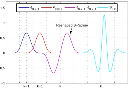
2.1. Boundary conditions. We want to maintain consistency the wavelets with boundary conditions of equation (1.1). To do this, we reshape every B-splines ϕj,k supported atx= 0 andx=m. Let,
ϕ0(x) =aϕj,−1(x) +bϕj,0(x) +cϕj,+1(x),
ϕm(x) =a′ϕj,2−jm−1(x) +b′ϕj,2−jm(x) +c′ϕj,2−jm+1(x).
Due to boundary conditions and (1.1),ϕ0 andϕm must satistify
ϕ0(0) = 0, ϕ ′′
0(0) = 0, ϕm(m) = 0, ϕ ′′
m(m) = 0.
The coefficients ofϕ0 andϕmcan be derived from these equations, so we have,
ϕ0(x) =ϕj,−1(x)−ϕj,+1(x),
The process for the B-spline wavelets is the same. We also described more complicated boundary conditions via wavelets in [3].
Figure 1. The cubic B-spline functions ϕ0, k−1 and ϕ0, k+1, the cubic
B-spline waveletψ0, kand the reshaped scaling function (ϕ0, k+1−ϕ0, k−1).
k−1 k+1 k k
−1 −0.5 0 0.5 1
1.5 φ0,k−1 φ0,k+1 φ0,k−1−φ0,k+1 ψ0,k
Reshaped B−Spline
3. The approximation for the stochastic evolution equation For the time discretization of equation (1.1) we use the implicitθ-Euler-Maruyama scheme. Leth= NT, be a time step, tn =nh, n= 0, . . . , N. We denote an approxi-mate solution of u(x, t) in the spaceVj−1 by uj(x, t). Using time stepping θ -Euler-Maruyama scheme, the SPDE (1.1) is written as
unj+1(x) =unj(x) +hA(θ unj+1(x) + (1−θ)unj(x))
+hf(unj+1(x)) +g(unj(x))∆Wn. (3.1)
For the grid pointsxi =i2j−1, i= 0,1, . . . , m2−j+1, let ukj = [ukj(x0), . . . , ukj(xN′)]. Now we put the matrix form of the differential operator A in the numerical (3.1), then we have
ujn−+11 =unj−1+hDjPj−−11(θunj−+11 + (1−θ)unj−1)
+hFnj−1+Gnj−1∆Wn, (3.2)
where Fnj = [f(unj(x0), . . . , f(unj(xN′))]T and Gnj = [g(u n
j(x0), . . . , g(unj(xN′))]T. Now, multiplying (3.2) by(Fj−1·Pj−−11
)
, we derive
[
an+1
bn+1 ]
=
[
an bn
]
+θMj−1 [
an+1
bn+1 ]
h+ (1−θ)Mj−1 [
an bn
] h
+h [
fn a fn
b
]
+
[
gn a gn b
]
where
[
fan fbn
]
=Fj−1·Pj−−11F
n j−1,
[
gna gnb,
]
=Fj−1·Pj−−11G
n
j−1, and Mj−1= [
A B
C D
] .
Therefore,
(I−θhMj−1) [
an+1
bn+1 ]
= (I+ (1−θ)hMj−1) [
an bn
]
+h [
fn a fn
b
]
+
[
gn a gn b
]
∆Wn. (3.4)
To increase the accuracy of the solution in some places of domain Ω and to avoid growing the calculations we use the multi-scale method. This means that we solve the system in a spaceVj and domain Ω which we call the large scale system (coarse resolution). Once again we solve the system in a finer space Vj−1 and subdomain
Λ that we call small scale system (fine resolution). Combination of the solutions of these two systems makes suitable accuracy and less computation than the solutions of the system achieved in the space Vj−1 on domain Ω. One can consider several
subdomains and solve the SPDE in different resolutions, but we consider a subdomain for simplicity. In fact, depending on the number of mentioned subdomains we have the same number of additional systems.
At first, for constructing large scale system, we don’t use all of the elements in
Mj−1. The elements ofMj−1 must be broken up into a block decomposition that is
compatible with the block structure of the vector
[
an bn
] .
We only consider the blockAover all domain Ω. Then using time stepping scheme (3.3), we find an approximation foran+1 via (3.5) which we callaT m
Λ
(I−θhA)an+1= (I+ (1−θ)hA)an+hfan+ gan∆Wn. (3.5)
In the next step, we solve the system on the subdomain Λ at the small scale resolution
Vj−1
( I−θh
[
A B
C D
])
Λ [
an+1 bn+1 ]
Λ
=
(
I+ (1−θ)h [
A B
C D
])
Λ [
an bn
]
Λ
+h [
fan fbn
]
Λ
+
[
gna gnb
]
Λ
∆Wn,
whereAΛ, BΛ, CΛ andDΛ are composed from the elements of A, B,C andD that
Now, we are looking for the vector correction aCr where an+1 = aT m+aCr. Consider theθ-Euler-Maruyama method for this case, sinceanΛ+1=aT mΛ +aCrΛ thus
(I−hθMj−1)Λ [
aCr
Λ
bnΛ+1
]
= (I+ (1−θ)hMj−1)Λ [ 0 bn ] Λ +h [ 0 fn a ] Λ + [ 0 gn a ] Λ
∆Wn
+
[
0
CΛ ] (
θhaT mΛ + (1−θ)hanΛ). (3.6)
By solving system (3.6), we get the vector
[
an+1
bn+1 ]
Λ
.
The last step is to construct the vector
[
an+1
bn+1 ]
Ω
from vectors
[
aT m 0
]
Ω
and
[
an+1 bn+1
]
Λ
. In the subdomain Λ, the vector
[
an+1 bn+1
]
Λ
is a better approximate
solution than the vector
[
aT m 0
]
Λ
for system (3.5). So to increase the accuracy of the
approximate vector
[
aT m 0
]
Ω
we must replace elements of
[
aT m 0
]
Ω
by the elements
of
[
an+1
bn+1 ]
Λ
, indeed we substitude the only ones that are related to subdomain Λ
a Tm 0 =
Xj0(Tm) .. .
aT m
Λ
.. .
XjN′(Tm)
0 .. . 0Λ .. . 0 ↔ and ↔
anΛ+1
bnΛ+1
Replace −−−−−→
Xj0(Tm) .. . anΛ+1
.. .
XjN′(Tm)
0 .. . bnΛ+1
.. . 0
≡
a
n+1
bn+1
. (3.7)
This completes the method.
As an example, let Ω = [0,10]. If one solves the problem in V−7, an involves
27(10) = 1280 elements . But in V
−6, the resolution of the large scale system has
26(10) = 640 coefficients. If our problem requires high resolution, inV
−7, in a
subdo-main such as Λ = [2.5,4.5], then small scale system has 27(4.5−2.5) = 256 coefficients.
So solving the small scale system and the large scale system inV−6 separately would
involve 896 elements which has less computational cost than solving the problem in whole domain Ω inV−7.
4. Stability and Consistency
In this section we consider the consistency and stability of the method, we recall the following definitions from [36].
Definition 4.1. (Consistency) A stochastic difference scheme Ln
kunk =Gnk is point-wise consistent with the SPDELu =G, if for any continuously twice differentiable function Φ in mean square
E∥(Lu−G)|nk−Lnku(k∆x, n∆t)−Gnk∥2∞→0, (4.1)
as ∆x→0 and ∆t→0.
Definition 4.2. (Stability) A stochastic difference scheme is said to be stable in mean square if there exist some positive constants ∆x0 and ∆t0 and non-negative
constantsK andβ such that
Eun+12 ∞≤Ke
βtEu02
∞, (4.2)
for all 0≤t= (n+ 1) ∆t, 0≤∆x≤∆x0, and 0≤∆t≤∆t0.
Theorem 4.3. Let ej(x)be the error of second derivative of approximation of Φ∈
C2[0, m] inV
j−1, we have
|ej(x)|=O
(
Proof. Assume that Φ is represented by (2.10), then let Taylor expansion of Φ ∈
C2[0, m] inx0∈[0, m], can be written
Φ(x) = Φ(x0) + (x−x0)Φ′(x0) +
(x−x0)2
2 Φ
′′(ζ), ζ∈D
Φ,
let x0 = 2jk and bj, k be the coefficient of representation Φ by expansion of cubic B-spline wavelet as (2.10). Then from (2.6) we have
bj,k=
∫ 2j−1(k+4)
2j−1(k−3)
Φ(x)ψej,k(x)dx
=
∫ 2j−1(k+4)
2j−1(k−3)
Φ(2jk)ψej,k(x) + (x−2jk)Φ′(2jk)ψej,k(x)dx
+
∫ 2j−1(k+4)
2j−1(k−3)
(x−2jk)2
2 Φ
′′(ζ)ψe
j,k(x)dx. (4.4)
Using (2.6) and substituting u = 2−jx−k in the above equation the first integral vanishes
bj,k=
∫ 2j−1(k+4)
2j−1(k−3)
(x−2jk)2 2 Φ
′′(ζ)ψej,k(x)dx. (4.5)
For allx= 2jl,0≤l≤m2−j, we have
|ej(x)|=
−∞ ∑
i=j m2−i−1
∑
k=0
bi,kψ′′i,k(x)
, (4.6)
ej(x)=
−∞ ∑
i=j m2∑−i−1
k=0 bi,k ∂2 ∂x2 √ 2∑ r
grϕi−1,r+k(x)
=√2
−∞ ∑
i=j m2∑−i−1
k=0 bi,k ∑ r gr ∂2 ∂x22
1−i
2 B3(21−ix−r−k)
.
From (2.4), we have
ej(x)= 8
−∞ ∑
i=j m2−i−1
∑
k=0
bi,k2−25i
∑
r
gr
(
B1(21−ix−r−k)
−2B1(21−ix−r−k−1) +B1(21−ix−r−k−2)
) = 8 −∞ ∑
i=j 2−25i
∑
r
gr m2−i−1
∑
k=0 bi,k
(
B1(21−ix−r−k)
−2B1(21−ix−r−k−1) +B1(21−ix−r−k−2)
)
sinceB1(21−i2jl−r−k) is nonzero only fork= 2j−i+1l−r, so we have
ej(2jl)= 8
−∞ ∑
i=j 2−25i
∑
r
grB(bi,s−2bi,s−1+bi,s−2)
,
wheres= 2j−i+1l−randB =B1(0). From (4.5) we get
ej(2jl)= 8B
−∞ ∑
i=j 2−25i
∑
r
gr
∫ 2i−1(s+4)
2i−1(s−3)
(x−2is)2
2 Φ
′′(ζ)ψe
i,s(x)dx
−2
∫ 2i−1(s+3)
2i−1(s−4)
(x−2i(s−1))2
2 Φ
′′(ζ)ψe
i,s−1(x)dx
+
∫ 2i−1(s+2)
2i−1(s−5)
(x−2i(s−2))2
2 Φ
′′(ζ)ψe
i,s−2(x)dx
. (4.8)
Thus
ej(2jl)≤8B
−∞ ∑
i=j
∑
r
gr|Φ′′(ζi,s)−2Φ′′(ζi,s−1) + Φ′′(ζi,s−2)|
×
∫ 4
−3 u2
2
eψ(u)du
, (4.9)
whereζi,s,ζi,s−1 andζi,s−2 are in [2i−1(S−5),2i−1(S+ 4)]. Since Φ is continuesly
twice differentiable we can considerj such that
|Φ′′(ζi,s)−2Φ′′(ζi,s−1) + Φ′′(ζi,s−2)|<2i, ∀i≤j <0,
finally from (4.9), we get
ej(2jl)≤8B2j+1
∑
r
gr
∫ 4
−3 u2
2
eψ(u)du. (4.10)
Now, we investigate the consistency of the proposed method.
Theorem 4.4. The stochastic scheme (3.4) is consistent in mean square.
Proof. Letφ(x, t) be a smooth function, and
L(φ)|nk =φ(k∆x,(n+ 1) ∆t)−φ(k∆x, n∆t)
−
∫ (n+1)∆t
n∆t
Aφ(k∆x, s)ds−
∫ (n+1)∆t
n∆t
f(φ(k∆x, s))ds
−
∫ (n+1)∆t
n∆t
We present (4.11) in the matrix form:
L(φ)|n= Φ ((n+ 1) ∆t)−Φ (n∆t)
−
∫ (n+1)∆t
n∆t
AΦ(s)ds−
∫ (n+1)∆t
n∆t ¯ F(s)ds
−
∫ (n+1)∆t
n∆t ¯
G(s)dW(s), (4.12)
where
L(φ)|n=
[
L(φ)|n1, L(φ)|n2, . . . , L(φ)|n2q
]T
,
Φn = Φ (n∆t) = [φ(∆x, n∆t), φ(2∆x, n∆t), . . . , φ(2q∆x, n∆t)]T ¯
F(s) = [f(φ(∆x, s)), f(φ(2∆x, s)), . . . , f(φ(2q∆x, s))]T ¯
Fn = [f(φ(∆x, nh)), f(φ(2∆x, nh)), . . . , f(φ(2q∆x, nh))]T. (4.13)
and ¯G, ¯Gn are the same as the definetion of ¯Fand ¯Fn for function g instead of f. On the other hand, from (3.2),
Lnφ= Φn+1−Φn−θhDj(Pj−1)− 1
Φn+1 −(1−θ)hDj(Pj−1)−
1
Φn
−hF¯n− G¯n∆Wn. (4.14) Then
E∥Lφ|n−Lnφ∥2∞< E
θ
∫ (n+1)∆t
n∆t
Dj(Pj−1)− 1
Φn+1− AΦ (s)ds
−(1−θ)
∫ (n+1)∆t
n∆t
Dj(Pj−1)− 1
Φn− AΦ (s)ds
−
∫ (n+1)∆t
n∆t ¯
Fn−F¯(s)ds
−
∫ (n+1)∆t
n∆t ¯
Gn−G¯ (s)dW(s)
∞
. (4.15)
From Lipschitz property off, boundedness of derivative ofg, and Theorem4.3, also from the square property of the Itˆo integral, we conclude
E∥LΦ|n−LnΦ∥2∞→0, n→ ∞. (4.16)
In the following we want to investigate stability of the solution (3.4) .
Lemma 4.5. The infinity norm of the matrix (Pj)−1 is bounded. In fact
(Pj)−1
∞≤2 j
Proof. We rewrite Pj= 2
−j
2 2
3(I+Q) whereQ= (qi k) is a tridiagonal with qi k=
{ 1
4, i=k±1,
0, o.w.
So (Pj)−
1
= 2j23
2
∞ ∑
k=0
(−1)kQk. Since∥Pj∥
∞= 2
−j
2 and∥Q∥
∞=12, we get
(Pj)−
1
∞≤2 j
23 2
∞ ∑
k=0
Qk
∞=2 j
23 2
1 1−1
2
= 2j23. (4.17)
Theorem 4.6. The stochastic scheme (3.2) approximating the solution of (1.1) is stable in mean square sense with respect to the∥ · ∥∞-norm.
Proof. From (3.2), we have
(
I−θhDj(Pj−1)− 1)
un+1=
(
I+ (1−θh)Dj(Pj−1)− 1)
un
+hF¯n+ ¯Gn∆Wn. (4.18) Choosehsmall enough such that
θhDj(Pj−1)− 1
∞≤
1
2 <1, (4.19)
Then the following matrix is invertible
I−θhDj(Pj−1)− 1
. (4.20)
Also we obtain
(I−θhDj(Pj−1)−
1)−1
∞≤
1 1−∥θhDj(Pj−1)−1∥
∞
≤2, (4.21)
Using (4.18) we have
Eun+12∞=E (
I−θhDj(Pj−1)− 1)−1
×((I+ (1−θ)hDj(Pj−1)− 1)
un+ ¯Fn+ ¯Gn∆Wn)
2
∞
. (4.22)
Due to the properties off andg we conclude
Eun+12∞≤
(
I −θhDj(Pj−1)−1
)−1
2
∞
×
(
1 + (1−θ)hDj(Pj−1)− 1
2
∞+c h )
E∥un∥2∞. (4.23)
Finally, using (4.23) and Lemma4.5, there is a positive constant Csuch that
Eun+12∞≤C E∥un∥2∞. (4.24)
According to the Theorems 4.4 and 4.6 and the stochastic version of the Lax-Richtmyer theorem [37,38], the stochastic method (3.4) is convergent to the solution of the stochastic parabolic partial differential equation (1.1).
5. Numerical Results
In this section we consider some SPDEs, and apply our numerical method to ap-proximate their solutions for different resolution levels. For each resulotion levelj
and choice ∆t, 10,000 runs are performed with different samples of the noise, and the averaged value Eun
j(x)−un−7(x) is calculated. Here we assume the approximate
solution inV−7 as the exact solution. The examples illustrate the convergence of the
numerical method and also they show that the approximate solutions satisfy in the boundary points exactly.
Example 5.1. Consider the following SPDE
du(x, t) =
( ∂2
∂x2u(x, t)−u 3(x, t)
)
dt+u(x, t)dW(t), (5.1)
u(x,0) = 10x(1−x), u(0, t) =u(1, t) = 0.
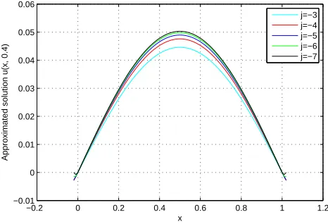
From Figure2and Table1it is obvious that the method is convergence. Furthermore, from Figure2we can see that the approximate solutions satisfy boundary conditions exactly.
Figure 2. Approximate solution of Example5.1in different resolutions at t=0.3.
−0.2 0 0.2 0.4 0.6 0.8 1 1.2
−0.01 0 0.01 0.02 0.03 0.04 0.05 0.06
x
Approximated solution u(x, 0.4)
Table 1. The errors are the difference between the results inVjand the results inV−7(denoted by Vj/V−7) withh= 0.01 att= 0.4,θ= 0.6, for
Example5.1.
V−3/V−7 V−4/V−7 V−5/V−7 V−6/V−7
ErrorL∞ 0.005706 0.002870 0.002639 0.001446 Error L2 0.004047 0.001949 0.000987 0.000413
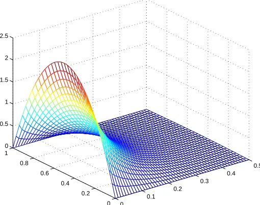
Figure 3. Approximate solution of Example5.1, inV−5 withh= 0.01.
0 0.1
0.2 0.3
0.4 0.5
0 0.2 0.4 0.6 0.8 1 0 0.5 1 1.5 2 2.5
Example 5.2. Consider the following SPDE
du(x, t) =
( ∂2
∂x2u(x, t) + sin(u(x, t)) )
dt+u2(x, t)dW(t), (5.2)
u(x,0) = sin(x), u(0, t) =u(1, t) = 0.
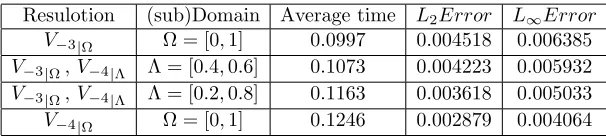
From Figure 5 and Table 2 it is obvious that the method is convergent. In Table
3, the numerically approximate errors of the different the multi-scale systems are compared with the full domainV−3 system and the full domainV−4 system. Here,
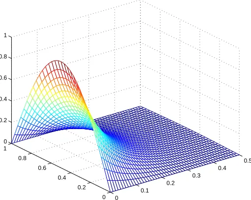
Figure 4. Approximate solution of Example5.2, inV−5 withh= 0.01.
0 0.1
0.2 0.3
0.4 0.5
0 0.2 0.4 0.6 0.8 1 0 0.2 0.4 0.6 0.8 1
Figure 5. Approximate solution of Example5.2in different resolutions att= 0.3.
−0.2 0 0.2 0.4 0.6 0.8 1 1.2
−0.005 0 0.005 0.01 0.015 0.02 0.025 0.03
x
Approximated solution u(x, 0.4)
j=−3 j=−4 j=−5 j=−6 j=−7
6. Conclusion
Table 2. The errors are the difference between the results inVjand the results inV−7(denoted by Vj/V−7) withh= 0.01 att= 0.4,θ= 0.6, for
Example5.2.
V−3/V−7 V−4/V−7 V−5/V−7 V−6/V−7
ErrorL∞ 0.006385 0.004064 0.002219 0.000908 Error L2 0.004518 0.002879 0.001576 0.000647
Table 3. The errors and computational time of the multi-scale systems for Example 5.2, compared with the results of a V−3 resolution single
system and results of a V−4 resolution single system with h = 0.01 at t = 0.4 andθ = 0.6. The computational time is the average computing time (in seconds) per time run.
Resulotion (sub)Domain Average time L2Error L∞Error V−3|Ω Ω = [0,1] 0.0997 0.004518 0.006385 V−3|Ω, V−4|Λ Λ = [0.4,0.6] 0.1073 0.004223 0.005932 V−3|Ω, V−4|Λ Λ = [0.2,0.8] 0.1163 0.003618 0.005033 V−4|Ω Ω = [0,1] 0.1246 0.002879 0.004064
evolution equations at different resolutions, in different domains. In this method, wavlets are reshaped to satisfy boundary conditions (1.1) exactly. Then by reducing the equation into two systems, it was found that the method requires less computa-tional cost than the high resolution results. The convergence of the method has been shown in this article. At last, numerical experiments have confirmed the efficiency of this method.
References
[1] E. J. Allen, S. J. Novosel, and Z. Zhang,Finite element and difference approximation of some linear stochastic partial differential equations, Stoch. Rep.,64(1998), 117–142.
[2] H. Aminikhah, M. Tahmasebi, and M. Mohammadi Roozbahani, Numerical solution for the time-space fractional partial differential equations using the wavelet multi-scale method, U. P. B. Sci. Bull., Series A,78(2016), 175–188.
[3] H. Aminikhah, M. Tahmasebi, and M. Mohammadi Roozbahani, The multi-scale method for solving nonlinear time space-fractional partial differential equations, IEEE J. Autom. Sinica, In press. DOI 10.1109/JAS.2016.7510058
[4] I. Babuˇska, R. Tempone, and G. E. Zouraris, Galerkin finite element approximations of sto-chastic elliptic partial differential equations, SIAM J. Numer. Anal.,42(2004), 800–825. [5] C. Blatter,Wavelets, A Primer, A K Peters/CRC Press, Florida, 2002.
[6] A. Cohen, I. Daubechies, and J.-C. Feauveau, Biorthogonal bases of compactly supported wavelets, Commun. Pure Appl. Math.,70(1992), 485–560.
[7] A. M. Davie and J. G. Gaines,Convergence of numerical schemes for the solution of parabolic stochastic partial differential equations, Math. Comp.,70(2001), 121–134.
[9] Q. Du and T. Zhang, Numerical approximation of some linear stochastic partial differential equations driven by special additive noises, SIAM J. Numer. Anal.,40(2002), 1421–1445. [10] M. Geissert, M. Kov´acs, and S. Larsson,Rate of weak convergence of the finite element method
for the stochastic heat equation with additive noise, BIT,49(1995), 343–356.
[11] W. Grecksch and P. E. Kloeden, Time-discretised Galerkin approximations of parabolic sto-chastic PDEs, Bull. Aust. Math. Soc.,54(1999), 79–85.
[12] I. Gy¨ongy and D. Nualart,Implicit scheme for quasi-linear parabolic partial differential equa-tions perturbed by spacetime white noise, Stochastic Process. Appl.,58(1995), 57–72.
[13] I. Gy¨ongy,Lattice approximations for stochastic quasi-linear parabolic partial differential equa-tions driven by space-time white noise I, Potential Anal.,9(1998), 1–25.
[14] I. Gy¨ongy,Lattice approximations for stochastic quasi-linear parabolic partial differential equa-tions driven by spacetime white noise II, Potential Anal.,11(1999), 1–37.
[15] I. Gy¨ongy and T. Mart´ınez, On numerical solution of stochastic partial differential equations of elliptic type, Stochastics,78(2006), 213–231.
[16] I. Gy¨ongy and A. Millet,Rate of convergence of space time approximations for stochastic evo-lution equations, Potential Anal.,30(2009), 29–64.
[17] E. Hausenblas, Numerical analysis of semilinear stochastic evolution equations in Banach spaces, J. Comput. Appl. Math.,147(2002), 485–516.
[18] E. Hausenblas,Approximation for semilinear stochastic evolution equations, Potential Anal., 18(2003), 141–186.
[19] E. Hausenblas,Finite element approximation of stochastic partial differential equations driven by Poisson random measures of jump type, Potential Anal.,46(2007/2008), 437–471.
[20] A. Jentzen,Pathwise numerical approximations of SPDEs with additive noise under non-global Lipschitz coefficients, Potential Anal.,145(2009), 375–404.
[21] A. Jentzen and P. E. Kloeden,Overcoming the order barrier in the numerical approximation of stochastic partial differential equations with additive space-time noise, Proc. R. Soc. Lond. Ser. A Math. Phys. Eng. Sci.,465(2009), 649–667.
[22] M. A. Katsoulakis, G. T. Kossioris, and O. Lakkis,Noise regularization and computations for the 1-dimensional stochastic Allen-Cahn problem, Interfaces Free Bound.,9(2007), 1–30. [23] P. E. Kloeden and S. Shott,Linear-implicit strong schemes for Ito-Galerkin approximations of
stochastic PDEs, J. Appl. Math. Stochastic Anal.,14(2001), 47–53.
[24] M. Kov´acs, S. Larsson, and F. Lindgren,Strong convergence of the finite element method with truncated noise for semilinear parabolic stochastic equations with additive noise, Numer. Algo-rithms,53(2010), 309–320.
[25] M. Kov´acs, F. Lindgren, and S. Larsson, Spatial approximation of stochastic convolutions, J. Comput. Appl. Math.235(2011), 3554–3570.
[26] M. Kov´acs, S. Larsson, and F. Saedpanah,Finite element approximation of the linear stochastic wave equation with additive noise, SIAM J. Numer. Anal.,48(2010), 408–427.
[27] M. Kov´acs, S. Larsson, and K. Urban,On Wavelet-Galerkin Methods for Semilinear Parabolic Equations with Additive Noise, In Monte Carlo and quasi-Monte Carlo methods 2012, Springer Proceedings in Mathematics and Statistics, Vol. 65, Springer, Berlin Heidelberg, (2013), 481– 499.
[28] G. J. Lord and J. Rougemont,A numerical scheme for stochastic PDEs with Gevrey regularity, IMA J. Numer. Anal.,24(2004), 587–604.
[29] G. J. Lord and T. Shardlow,Postprocessing for stochastic parabolic partial differential equations, SIAM J. Numer. Anal.,45(2007), 870–889.
[30] D. A. McLaren,Sequential and localized implicit wavelet-based solvers for stiff partial differential equations, Thesis (Ph.D.)–University of Ottawa, Ottawa, Canada, 2012.
[31] A. Millet and P. L. Morien,On implicit and explicit discretization schemes for parabolic SPDEs in any dimension, Stochastic Process. Appl.,115(2005), 1073–1106.
[33] T. M¨uller-Gronbach, K. Ritter, and T. Wagner,Lower bounds and nonuniform time discretiza-tion for approximadiscretiza-tion of stochastic heat equadiscretiza-tions, In Monte Carlo and quasi-Monte Carlo methods 2006. Springer, Berlin, (2007), 577–589.
[34] T. M¨uller-Gronbach, K. Ritter, and T. Wagner,Optimal pointwise approximation of infinitedi-mensional Ornstein-Uhlenbeck processes, Stoch. Dyn.,8(2008), 519–541.
[35] R. Pettersson and M. Signahl,Numerical approximation for a white noise driven SPDE with locally bounded drift, Potential Anal.,82(2005), 375-393.
[36] C. Roth,Difference methods for stochastic partial differential equations, ZAMM. Z. Angew. Math. Mech.,82(2002), 821-830.
[37] C. Roth,First Order Stochastic Partial Differential Equations, Thesis (Ph.D.)–Martin-Luther University Halle-Wittenberg, Halle, 2002.
[38] C. Roth,A Combination of Finite Difference and Wong-Zakai Methods for Hyperbolic Stochas-tic Partial Differential Equations, Stoch. Anal. Appl.,24(2006), 221–240.
[39] C. Roth,Weak approximations of solutions of a first order hyperbolic stochastic partial differ-ential equation, Monte Carlo Methods Appl.,13(2007), 117–133.
[40] C. Schwab and R. Stevenson,Space-time adaptive wavelet methods for parabolic evolution prob-lem, Math. Comp.,78(2009), 1293–1318.
[41] T. Shardlow,Numerical methods for stochastic parabolic PDEs, Numer. Funct. Anal. Optim., 20(1999), 121–145.
[42] J. B. Walsh,Finite element methods for parabolic stochastic PDEs, Potential Anal.,23(2005), 1–43.
[43] J. B. Walsh,On numerical solutions of the stochastic wave equation, Illinois J. Math.,50(2006), 991–1018.
[44] X. Wang and G. Jiang, Lp-strong solutions of stochastic partial differential equations with monotonic drifts, J. Math. Anal. Appl.,415(2014), 178–203.
[45] Y. Yan,Semidiscrete Galerkin approximation for a linear stochastic parabolic partial differential equation driven by an additive noise, BIT,44(2004), 829–847.
[46] Y. Yan,Galerkin finite element methods for stochastic parabolic partial differential equations, SIAM J. Numer. Anal.,43(2005), 1363–1384.