Numerical solution of optimal control problems by using a new
sec-ond kind Chebyshev wavelet
Mehdi Ramezani
Department of mathematics, Tafresh University, Tafresh 39518 79611, Iran.
E-mail: [email protected]
Abstract The main purpose of this paper is to propose a new numerical method for solving the optimal control problems based on state parameterization. Here, the boundary conditions and the performance index are first converted into an algebraic equation or in other words into an optimization problem. In this case, state variables will be approximated by a new hybrid technique based on new second kind Chebyshev wavelet.
Keywords. Second kind chebyshev wavelet, optimal control problems, numerical analysis.
2010 Mathematics Subject Classification. 65L05, 34K06, 34K28.
1. Introduction
To achieving an optimal control for the considered problems is not a simple task. Recently, optimal control is introduced as a mathematically challenging and practi-cally important discipline [1,2] . Traditional control techniques are based on model constructions. However, it may be difficult to construct an accurate enough model or to employ a lot of assumptions to solve a differential equation. There exist also several optimal control problems which are subject to constraints in state and/or control vari-ables. Direct methods can obtain the optimal solution by direct minimization of the cost function (performance index), subject to constraints. Among these approaches, Pontryagins maximum principle method and dynamic programming introduced the best known methods for solving the optimal control problems [3, 4, 5, 6, 7,8]. Be-cause analytical solutions for optimal control problems cant always be solved acces-sible, finding an approximate solution can be a good idea to solve them. Numerical approaches have provided a personable field for researchers to the appearance of dif-ferent numerical computational methods and efficient algorithms for solving optimal control problems (for details see [9,10]). In this study, the Chebyshev wavelet method in [11,12] is modified by the second kind Chebyshev, and an impressive iterative al-gorithm is proposed. In this method, only one unknown coefficient is achieved for finding a proper approximation; further iterations result better accuracy.
Received: 28 November 2016 ; Accepted: 13 December 2016.
2. Second Kind Chebyshev Wavelet
Generally, wavelets functions are generated from translation and dilation of a def-inite function called mother wavelet [11, 12, 13]. By considering the translation pa-rameter (b) and dilation parameter (a) with a normalized time (t), wavelet functions can be described as below
Ψab(t) =|a| −1
2Ψ t−b
a
, a, b∈R, a6= 0 , (2.1)
Consider the second kind Chebyshev wavelets as Ψ(t) = Ψ(m, n, t) where n = 1,2, ...,2k(k = 0,1,2, ...) and m illustrates the order of the second kind Chebyshev
polynomial [12, 14, 15,16, 17, 18]. By considering the illustrated cases, the hybrid second kind Chebyshev wavelet can be given as below
Ψnm(t) = (
αm2 k
2 √
π Tm(2
k+1t−2n+ 1), n−1 2k ≤t≤
n 2k,
0, o.w. (2.2)
where
αm(t) = √
2, m= 0,
2, m= 1,2, . . . . (2.3)
In the equation above, Tm(t) describes the second kind orthogonal Chebyshev
polynomial of order m , [14, 19]. the orthogonality can be proved by the weight functionw(t) = √1
1−t2 . The second kind Chebyshev polynomial can be presented as
a three part recursive formula [12]
T0(t) = 1,
T1(t) = 2t,
..
. , t∈[−1,1],
Tn(t) = 2tTn−1(t)−Tn−2(t).
(2.4)
Therefore, the total Chebyshev wavelet approximation can be considered as below:
f(t)'
∞ X n=1 ∞ X m=0
fnmΨnm(t). (2.5)
If the infinite series in Eq. 2.5are truncated, then Eq. 2.5can be written as
f(t)'
2k X n=1 m−1 X m=0
fnmΨnm(t). (2.6)
wn(t) =w(2k+1t−2n+ 1). (2.7)
3. Solving Optimal Control Problems
Lets consider a nonlinear state equation as below [20],
u(τ) =f(τ, x(τ),x(τ)),˙ (3.1)
where the initial conditions are:
x(t0) =x0, x(t1) =x1, (3.2)
here, u(.) : [t0, t1] → R and x(.) : [t0, t1] → R are the signal control and state variables respectively and f describes the continuously differentiable function with real-value. The main purpose of the optimal control problem is to minimize a definite performance index (PI) by achieving a proper control signal from the initial position x(t0) =x0 to the final positionx(t1) =x1 within the time (t1−t0) ,
P I=
t1 Z
t0
L(τ, x(τ), u(τ))dτ . (3.3)
Ift06= 0 ort16= 1 , then for solving the problem with the second kind Chebyshev
wavelet polynomials, we need the transformation below,
τ= (t1−t0)t+t0, (3.4)
after the conversation above, the optimal control variable, the initial conditions of the trajectoryx(t) and the performance index will be changed into:
u(t) =f((t1−t0)t+t0, x(t),x(t))˙ , (3.5)
x(0) =x0, x(1) =x1, (3.6)
J(x) = (t1−t0) 1 Z
−1
L((t1−t0)t+t0, x(t), u(t))dt. (3.7)
By considering Eq. (2.2) withk= 0 and the second kind Chebyshev wavelet basis as Ψm(t) = Ψ1m(t) , the approximation forx(.) can be achieved as below
x1(t) = 2 X
m=0
amΨm(t). (3.8)
x1(0) =π2(a0−a1+a2),
x1(1) =π2(a0+a1+a2),
(3.9)
the unknown coefficientsa0anda1, can be evaluated as below
a0=pπ4(x1+x0)−a2,
a1=pπ4(x1−x0),
(3.10)
so from Eq. (3.8) we obtain
x1(t) = √π
4 (x1+x0)−a2
Ψ0(t) + √π
4 (x1−x0)
Ψ1(t) +a2Ψ2(t). (3.11)
The above equations give us a chance to have just one uncertainty (a2). Since, a
robust approach has been performed. In the following,x2(t) can be approximated by
x2(t) =x1(t) + 3 X
m=1
amΨm(t). (3.12)
By substituting the boundary conditionsx2(0) =x1(0) =x0and x2(1) =x1(1) =
x1 , we have
a1Ψ1(0) +a2Ψ2(0) +a3Ψ3(0) = 0,
a1Ψ1(1) +a2Ψ2(1) +a3Ψ3(1) = 0,
(3.13)
then unknown coefficientsa1 anda2are as
a1=
Ψ2(0)Ψ3(1)−Ψ2(1)Ψ3(0)
Ψ1(0)Ψ2(1)−Ψ1(1)Ψ2(0)
a3,
a2=
Ψ1(0)Ψ3(1)−Ψ1(1)Ψ3(0)
Ψ1(1)Ψ2(0)−Ψ1(0)Ψ2(1)
a3.
(3.14)
Assuminga∗ as the minimizer of the performance indexP I(a3), P I(a∗) includes
the optimal control problem solution. Control and state variables can be also eval-uated from a∗ approximately. By considering the recurrence characteristics of the orthogonal functions, the more recurrence results the more precision. Lets assume the (n+ 1)thstep approximation in below
xn+1(t) =xn(t) + n+2 X
m=n
amΨm(t). (3.15)
By considering the boundary condition xn+1(0) = xn(0) = x0 and xn+1(1) =
an+2Ψn+2(0) +an+1Ψn+1(0) +anΨn(0) = 0, (3.16)
an+2Ψn+2(1) +an+1Ψn+1(1) +anΨn(1) = 0. (3.17)
Assuming the Eqs. (3.16) and (3.17), the unknown coefficients an and an+ 1 , can
be evaluated as below
an =
Ψn+1(0)Ψn+2(1)−Ψn+1(1)Ψn+2(0)
Ψn(0)Ψn+1(1)−Ψn(1)Ψn+1(0)
an+2, (3.18)
and
an+1=
Ψn(0)Ψn+2(1)−Ψn(1)Ψn+2(0)
Ψn(1)Ψn+1(0)−Ψn(0)Ψn+1(1)
an+2. (3.19)
By considering the above equations, the final recursive solution for the state vari-able is
xn+1(t) =xn(t) +an+2Ψn+2(t)
+Ψn(0)Ψn+2(1)−Ψn(1)Ψn+2(0) Ψn(1)Ψn+1(0)−Ψn(0)Ψn+1(1)
an+2Ψn+1(t)
+Ψn+1(0)Ψn+2(1)−Ψn+1(1)Ψn+2(0) Ψn(0)Ψn+1(1)−Ψn(1)Ψn+1(0)
an+2Ψn(t),
(3.20)
after evaluation the Eq. (3.18), the recursive will be stopped when
|en+1−en|< ε, (3.21)
as
en+1=P I(a∗n+1). (3.22)
4. Case Study
Assume the following example to minimize byu(t) using
J=
1 Z
0
x(τ)−1 2u(τ)
2
dτ, τ ∈[0,1], (4.1)
u(τ) = ˙x(τ) +x(τ). (4.2)
Also, the boundary conditions are
x(0) = 0, x(1) = 12(1−1 e)
2
. (4.3)
Here, the analytical solution can be achieved by the Pontryagin’s maximum prin-ciple as below [6]
x(τ) = 1−1 2e
τ−1+ 1
2e −1
e−τ, (4.4)
u(τ) = 1−eτ−1, (4.5)
by using Eqs. (3.18) and (3.19) , we have
x1(t) = 9.027033336764101a2t2+ 9.027033336764101a2t+ 0.199788200446864t,
(4.6)
u1(t) = 0.199788200446864t+ 9.027033336764101(a2t2+a2t−a2)
+0.199788200446864. (4.7)
By substituting Eqs (4.6) and (4.7) into Eq. (4.1) we have
J(a2) =−14.939343991559241a22 - 1.354214327316854a2+ 0.053326221012670.
(4.8)
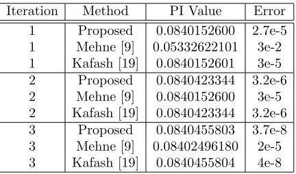
Table 1. Optimal cost functional J (PI) for differentnin case study.
Iteration Method PI Value Error
1 Proposed 0.0840152600 2.7e-5 1 Mehne [9] 0.05332622101 3e-2 1 Kafash [19] 0.0840152601 3e-5 2 Proposed 0.0840423344 3.2e-6 2 Mehne [9] 0.0840152600 3e-5 2 Kafash [19] 0.0840423344 3.2e-6 3 Proposed 0.0840455803 3.7e-8 3 Mehne [9] 0.08402496180 2e-5 3 Kafash [19] 0.0840455804 4e-8
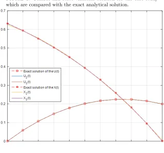
Figure 1. Control and state variables solution for the case study which are compared with the exact analytical solution.
5. Conclusion
In this research, a new and robust algorithm is proposed for the optimal control problems. The proposed method is a hybrid second kind Chebyshev and wavelet function which has good characteristics of both functions. The basis of the approach is on state parameterization and because of reducing the uncertainties in the problem, it gives robust results toward the other methods. The system performance is compared by two different methods and gives better results for a selected case study.
References
[1] D. Kirk,Optimal Control Theory: An Introduction, Prentice-Hall, Englewood Cliffs, NJ, 1970. [2] R. F. Stengel ,Optimal control and estimation. Courier Corporation, 2012.
[3] J. E. Rubio.,Control and Optimization: The Linear Treatment of Non-linear Problems, Manch-ester University Press, ManchManch-ester., 1986.
[4] B. D. Craven,Control and Optimization, Chapman & Hall, London, 1995.
[5] K. L. Teo, C. J. Goh and K. H. Wong,A Unified Computational Approach to Optimal Control Problems, Longman Scientific and Technical, England, 1991.
[6] LS. ,Pontryagin Mathematical theory of optimal processes. CRC Press, 1987.
[8] N. Razmjooy, M. Khalilpour, M. Ramezani, A New Meta-Heuristic Optimization Algorithm Inspired by FIFA World Cup Competitions: Theory and Its Application in PID Designing for AVR System, J. Control, Automation and Electrical Systems,27(4)(2016), 419–440.
[9] H. H. Mehne, and B. Hashemi ,A numerical method for solving optimal control problems using state parametrization, Num. Alg.,42(2006), 165–169.
[10] E. Nvdal,Solving continuous-time optimal-control problems with a spreadsheet. The J. of Eco-nomic Education,34(2)(2003), 99–122.
[11] M. Mahalakshmi and G. Hariharan,An efficient Chebyshev wavelet based analytical algorithm to steady state reactiondiffusion models arising in mathematical chemistry, J. Math. Chem.,
54(1)(2016), 269–285.
[12] N. Razmjooy and M. Ramezani.Analytical Solution for Optimal Control by the Second kind Chebyshev Polynomials ExpansionIranian J. Sci. and Tech. (Sciences) (2016), in press. [13] M. Lakestani, M. Jokar, M. Dehghan,Numerical solution of nthorder integrodifferential
equa-tions using trigonometric wavelets, Math. Methods in the App. Sci.,34(11)(2016), 1317–1329. [14] A. Saadatmandi, J. A. Farsangi.Chebyshev finite difference method for a nonlinear system of
second-order boundary value problems, App. Math. and Comp.,192(2)(2007), 586–591. [15] A. Saadatmandi, M. R Azizi, Chebyshev finite difference method for a TwoPoint Boundary
Value Problems with Applications to Chemical Reactor Theory, Iranian J. Math. Chem.,3(1)
(2012), 1–7.
[16] A. Saadatmandi, M. Dehghan,Numerical solution of hyperbolic telegraph equation using the Chebyshev tau method, Numerical Methods for Partial Differential Equations, 26(1) (2010), 239–252.
[17] A. Saadatmandi, M. Dehghan,The numerical solution of problems in calculus of variation using Chebyshev finite difference method, Phys. Lett. A,372 (22)(2008), 4037–4040.
[18] M. Razzaghi, S. Yousefi,The Legendre wavelets operational matrix of integration, Int. J. Sys. Sci.,32 (4)(2001) , 495–502
[19] B. Kafash, A. Delavarkhalafi and S. M. Karbassi.,Application of Chebyshev polynomials to derive efficient algorithms for the solution of optimal control problems, Sci. Iranica,19(3)(2012), 795– 805.