Development of the Distributed Points Method with Application to Cavitating Flow

University of New Orleans University of New Orleans

ScholarWorks@UNO

ScholarWorks@UNO

University of New Orleans Theses and

Dissertations Dissertations and Theses

12-19-2008

Development of the Distributed Points Method with Application to

Development of the Distributed Points Method with Application to

Cavitating Flow

Cavitating Flow

David M. Bourg

University of New Orleans

Follow this and additional works at: https://scholarworks.uno.edu/td

Recommended Citation Recommended Citation

Bourg, David M., "Development of the Distributed Points Method with Application to Cavitating Flow" (2008). University of New Orleans Theses and Dissertations. 904.

https://scholarworks.uno.edu/td/904

Development of the Distributed Points Method

with Application to Cavitating Flow

A Dissertation

Submitted to the Graduate Faculty of the University of New Orleans

in partial fulfillment of the requirements for the degree of

Doctor of Philosophy in

Engineering and Applied Science

by

David M. Bourg

B.S. University of New Orleans, 1992 M.S. University of New Orleans, 1993

ACKNOWLEDGMENTS

TABLE OF CONTENTS

Chapter 1 ...1

Introduction...1

Background and Motivation...2

Smoothed Particle Hydrodynamics...2

Initial Tests ... 10

Flow past rectangular obstruction...11

Flow through narrow gap ...14

Breaking dam ...16

Methods for Dealing with Cavity Flow... 19

Chapter 2 ... 23

The Distributed Points Method (DPM)... 23

Governing Equations ... 26

Gradient Computation ... 30

Least Squares Fit... 34

Standard Least Squares Algorithm... 34

Bi-quadratic Shape Function Solved Directly... 35

Plane Equation Shape Function... 41

Two-part Polynomial Shape Functions... 43

Weighting Function... 45

Numerical Implementation ... 49

Boundaries... 51

Viscosity... 52

Nearest Neighbor Search... 52

Time Stepping... 55

Chapter 3 ... 57

Initial tests of The Distributed Points Method... 57

Poiseuille Flow ... 57

Lid Driven Cavity ... 63

Multi-fluid Test ... 67

Chapter 4 ... 74

2D Circular Cylinder Benchmark ... 74

Baseline Test... 75

Parametric Tests ... 79

Downstream Length Sensitivity... 80

Blockage Sensitivity... 81

State Equation Sensitivity... 81

Weight Function Sensitivity... 82

Artificial Mach Number Sensitivity... 82

Reynolds Number Test Results ... 84

Chapter 5 ... 88

Extension to Multiphase flow ... 88

Single Phase State Equation ... 89

Multiphase State Equation... 92

The Equations...95

Discussion of Parameters...97

Chapter 6 ... 101

Cavitating flow numerical experiements ... 101

Circular Cylinder Tests ... 101

Flat Plate Tests... 105

Wedge Model ... 110

Cavity Length ... 111

Cavity Pinch... 113

Towards the Future... 118

References ... 120

Appendix ... 128

Selected Source Code... 128

TakeStep... 128

ComputeAllFields_RK4... 130

IntegrateContinuityEquation... 135

ComputePressures... 135

IntegrateMomentumEquations... 136

GetGradients... 137

ComputeGradientsBiQuadraticNormalEquations ... 140

ComputeGradientsPlaneNormalEquations ... 143

LIST OF FIGURES

Figure 1.1: Flow past obstruction initial wake formation ... 12

Figure 1.2: Wake development... 13

Figure 1.3: Further wake development with eddies ... 14

Figure 1.4: Piston driven flow through gap ... 15

Figure 1.5: Formation of “cavities”... 15

Figure 1.6: Initial particle configuration and start of motion ... 17

Figure 1.7: Fluid impacting container wall... 17

Figure 1.8: Fluid breaking back on itself ... 18

Figure 1.9: Initial secondary splash created by fluid-fluid impact... 18

Figure 2.1: Illustration of Eulerian Approach ... 28

Figure 2.2: Illustration of Lagrangian Approach... 29

Figure 2.3: Illustration of weighted interpolation ... 31

Figure 2.4: Two-part shape functions... 44

Figure 2.6: Gaussian function... 47

Figure 2.7: Linear weight function... 48

Figure 2.8: Background grid... 54

Figure 3.1: Poiseuille flow between two flat plates... 58

Figure 3.2: Lagrangian model ... 59

Table 3.1: Poiseuille flow parameters... 59

Figure 3.3: Lagrangian model, Re = 10.0 ... 60

Figure 3.4: Eulerian model results, Re = 10 ... 61

Figure 3.5: Poiseuille flow results comparison ... 62

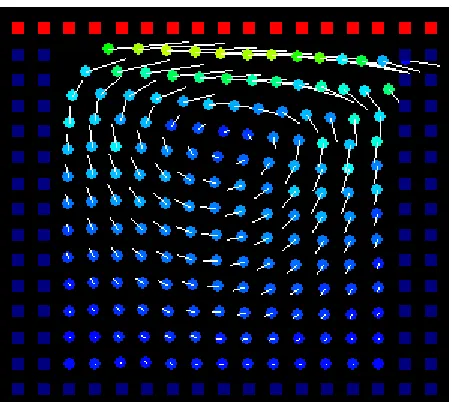
Figure 3.6: Lid driven cavity illustration ... 63

Figure 3.7: Lid driven cavity set up ... 64

Figure 3.8: Lagrangian test results... 65

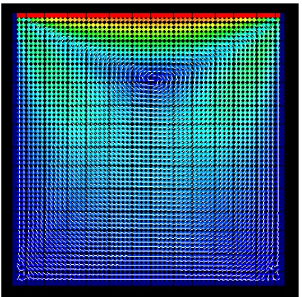
Figure 3.9: Lid driven cavity Eulerian model velocity plot ... 66

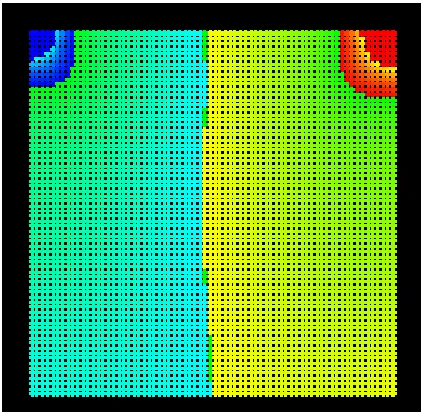
Figure 3.10: Lid driven cavity Eulerian model pressure plot... 67

Figure 3-11: Mulit-fluid test initial set up ... 68

Figure 3-12: Multi-fluid test initial set up with tracker particles... 68

Table 3.2: Multi-fluid flow parameters... 69

Figure 3-12: Density interpolation example... 70

Figure 3-13: Multi-fluid results... 71

Figure 3-14: Droplet density plots... 72

Figure 4-15: Settled fluid ... 73

Figure 4.1: Circular cylinder problem geometry... 75

Figure 4.4: Baseline test drag coefficient time history...78

Figure 4.5: Zoomed-in drag coefficient time history ... 79

Figure 4.6: Parametric test drag coefficient time histories ... 80

Figure 4.7: Extended domain downstream... 81

Figure 4.9: Test 8 drag coefficient power spectrum... 84

Figure 9: Drag coefficient results... 87

Figure 5.1: Barotropic state equation graph... 90

Figure 5.2: State equation graphs for various Mach numbers... 91

Figure 5.3: Multiphase state equation... 93

Figure 5.4: Effective sound speed ... 94

Figure 5.5: Effective Mach number ... 95

Figure 5.6: Multiphase state equation with γ = 7... 98

Figure 5.7: Effect of cavitation factor... 99

Figure 6.1: Cavity formation behind circular cylinder...102

Figure 6.2: Formed cavity behind circular cylinder ...102

Figure 6.3: Pinched bubble at cavity trailing edge. ...103

Figure 6.4: Pressure field at instant of pinch ...103

Figure 6.5: Velocity field at instant of pinch...104

Figure 6.6: Close-up of velocity field ...104

Figure 6.7: Flat plate density field, 88s...106

Figure 6.8: Flat plate density field, 97s...107

Figure 6.9: Pressure field at 88s...108

Figure 6.10: Velocity field...108

Figure 6.11: Velocity vector field ...109

Figure 6.12: Supercavitating wedge ...110

Figure 6.13: Cavity length comparison ...112

Figure 6.14: Cavity at 107.5 seconds ...113

Figure 6.15: Cavity at 112 seconds ...114

Figure 6.16: Cavity at 113.5 seconds ...114

Figure 6.17: Cavity pinch sequence ...115

Figure 6.18: Pressure field at instant after bubble implosion ...116

ABSTRACT

A mesh-less method for solving incompressible, multi-phase flow problems has been developed and is discussed along with the presentation of benchmark results showing good agreement with theoretical and experimental results. Results of a systematic, parametric study of the single phase flow around a 2D circular cylinder at Reynolds numbers up to 1000 are presented and discussed. Simulation results show good agreement with experimental results. Extension of the method to deal with multiphase flow including liquid-to-vapor phase transition along with applications to cavitating flow are discussed. Insight gleaned from numerical experiments of the cavity closure problem are discussed along with recommendations for additional research. Several conclusions regarding the use of the method are made.

C h a p t e r 1

INTRODUCTION

The original aim of this research effort was to develop a Smoothed Particle Hydrodynamics (SPH) -based method for simulating unsteady cavitating flow. It was intended that the resulting code would yield new improvements to the SPH method and would provide a new method for simulating unsteady cavitating flow. At the start of this effort in early 2005, an extensive literature survey was conducted that led to the conclusion that simulation of cavitating flow using SPH has never been attempted. An additional aim of this research was to further our understanding of the physics relevant to cavitating flow, specifically supercavitating flow.

The original research plan as detailed in my dissertation prospectus presented to my advisory committee in early 2005 made the statement “As with any new research effort I may encounter unanticipated difficulties or surprises that would require redirecting some effort. I’ve attempted to foresee what areas will require most attention; however, I’ve also kept the work plan flexible enough to allow adapting the plan as needs arise.” Indeed it wasn’t very long into my research effort that one of the most unanticipated events struck – Hurricane Katrina – that resulted in a virtual halt to my research plan.

their own errors and limitations, which themselves could conceivably require additional workarounds to deal with approximation errors. Instead of heading down that path I decided with my advisor at the time, Dr. Robert Latorre who has since retired from the University, to take a fresh look at the root of SPHs difficulty, namely, the very foundation of the method, it’s interpolation scheme.

This refocused effort has yielded an SPH inspired method I call the Distributed Particle Method

(DPM), which, like SPH, is a meshless method for solving the Navier-Stokes equations. The DPM retains the key benefits of SPH. Further, as originally aimed for, I extended the DPM method to deal with cavitating flow.

This document provides an overview of my research effort summarizing the SPH method as a basis for the DPM method, development and benchmarking of the DPM method for single phase flow, and extension of the DPM method to cavitating flow. The remainder of this chapter gives an overview of the SPH method along with motivation for development of a meshless method capable of handling cavitating flow. Chapter 2 covers details of the DPM as inspired by the SPH method. The next chapter, Chapter 3, describes and presents results for several initial numerical experiments using the DPM. Chapter 4 presents discussion and results for further benchmarking the DPM for 2D flow around a circular cylinder. Chapter 5 explains how the single phase DPM method was extended to treat multi-phased flow in order to simulate the liquid-to-vapor phase transition in cavitating flow. Finally, Chapter 6 presents results from several numerical experiments conducted using the multi-phase DPM.

Background and Motivation

Smoothed Particle Hydrodynamics

solid impact problems. This adaptability is truly a testament to the method’s generalized nature and versatility.

SPH is a meshless, Lagrangian particle method that is capable of handling free surface problems just as easy, if not easier, than internal flow problems. SPH was originally developed for boundless problems and treatments of rigid boundary conditions were added to the method over many years of development and adaptation to a variety of problems. That said, rigid boundaries still remain one of the more challenging aspects of implementing SPH owing to the truncation error, among other phenomenon, that results when field variables are interpolated over disparate points asymmetrically located adjacent to a rigid boundary.

Because SPH is a particle-based method instead of a mesh-based method, it is easier to code, especially for free surface problems where mesh entanglement is a serious issue with mesh-based methods. In SPH, once the governing equations are developed for the fluid(s) involved, the solution comes down to integrating the equations of motion for a number of particles representing the fluid(s). Implementation of SPH becomes more difficult when CPU usage optimization is required. Naive implementations of SPH result in tremendous computation requirements as the method is an N-Body method where, theoretically, every particle depends upon every other particle in the simulation. Thus,

computationally speaking the method scales as O(N2_{) as the number, N, of particles is increased.}

There are several approaches taken in practice to reduce the complexity to something approaching O(2N). (These approaches involve using kernels with compact support and implementation of optimized nearest neighbor search algorithms.)

The method of SPH is explained in detail in references [11], [13], and [14], among others, so I won’t repeat all the details here. However, I’ll give a brief overview of the fundamental principles of the method.

In SPH, the integral interpolant of a function A(r) is defined by the following:

∫

= ( ') ( ', ) '

)

(r A r W r r h dr A

or,

∑

=

j

j j

j

j W r r h

A m r

A( ) ( , )

ρ

where m is the mass of particle j, A is the value of any quantity of interest, rj is the position

vector of particle j, ρj is the density of particle j, and W is the interpolation kernel which is a function of r and h. Here h is the so-called smoothing length, which is ½ the radius which defines the circle encompassing nearest neighbors for a given particle. The smoothing length defines the support domain for the interpolation kernel of compact support. Another way of looking at the smoothing length is as the equivalent to the grid-scale of mesh-based methods.

The kernel interpolation function is typically Gaussian, or a close approximation, where only particles located within the smoothing circle contribute to the value of a quantity for a given particle. All particles falling outside this circle don’t contribute. This is key to optimizing the SPH method in terms of CPU usage as will be discussed later. (The Gaussian interpolation kernel does not have compact support; therefore, other kernels have been designed for specific applications that approximate the Gaussian but possess compact support.)

What’s clever about this method is that the kernel is an explicit function that can be differentiated analytically. This means that gradients of quantities of interest can be expressed in terms of the gradient of the kernel as follows:

∑

= ∇

j

j j

j

j W r r h

A m r

A( ) ( , )

ρ

kernel well enough but possess compact support and possess continuous first and second (or higher in some cases) derivatives.

Many different forms of the SPH interpolation kernel are in use these days and [24] describes specific requirements that must be fulfilled when designing an interpolation kernel.

For illustration purposes, I’ve included the cubic spline formulas here since this kernel seems to be the most widely used:

(

)

( ₂ 3

3 2 2 s s s h s s s h h r W σ σ where, h r s= π σ 7 10 =

As you can see, this kernel is effective for a distance of 2h around the particle under

consideration. Any particles falling outside this radius will not contribute to the interpolation.

SPH allows various equations of state for the fluid(s) under consideration. For incompressible flow problems the following equations of state have been used:

⎥ ⎥ ⎦ ⎤ ⎢ ⎢ ⎣ ⎡ − ⎟⎟ ⎠ ⎞ ⎜⎜ ⎝ ⎛ = 1 2 γ ρ ρ γ ρ o o c P

Here, P is the dynamic pressure of the particle under consideration, c is the speed of sound, ρo

is the reference (typically the initial) density, γ is the specific heat ratio, and ρ is the current density of the smoothed particle.

In SPH, pressure is an explicit function of density as you can see from the above equations. Recall that originally SPH was developed for compressible flow problems, thus to apply the method to

incompressible flow problems, you have to use an artificial speed of sound, c, such that density

variations are kept to about 1% to 3%; this gives a Mach number based on the maximum expected fluid velocity of about 0.1. Monaghan has shown, through analysis of the Navier-Stokes equations that the proper choice of c can be obtained from the following:

⎥ ⎥ ⎦ ⎤ ⎢ ⎢ ⎣ ⎡ ⎟ ⎠ ⎞ ⎜ ⎝ ⎛ ⎟⎟ ⎠ ⎞ ⎜⎜ ⎝ ⎛ ⎟ ⎟ ⎠ ⎞ ⎜ ⎜ ⎝ ⎛ = δ δ υ δ o o o o FL L V V

c max , ,

2 2 where o ρ ρ δ =Δ

Here, V_o is the velocity scale, L_o is the length scale, F is the body force per unit mass acting on the fluid, and ν is the kinematic viscosity.

Recently, truly incompressible versions of the SPH method have been introduced [25]. These versions eliminate the state equation and instead solve a Poisson equation to obtain pressure. Further, these versions require intermediate steps to evolve particle motions and then correct resulting velocities to yield a divergence free velocity field.

∑

i mW

1 ρ

Here, the density of particle i is found by interpolating over all other particles j. While this formula is simple in form and conserves mass, it does require multiple iterations over all particles before each integration time step in order to determine the density of each particle. A more computationally efficient approach is to use the SPH form of the continuity equation and evolve particle density during the simulation:

∑

Here, v is the particle velocity. This equation allows you to update the density (starting from an initial density) of each particle at each time step, thus it does not require extra iterations through the entire list of particles as does the previous equation for density. That said, this method of calculating density does not conserve mass exactly.

The SPH form of the momentum equation, without viscosity, is as follows:

ij i i i j j N j j i W P P m dt dv ∇ ⎟ ⎟ ⎠ ⎞ ⎜ ⎜ ⎝ ⎛ + − =

∑

=1 ρ 2 ρ 2

This is essentially the SPH version of Euler’s equation for a fluid particle. Fluid particles are driven by pressure gradients as you can see from the above equation. This equation is symmetric in that the pressure gradients result in equal and opposite central forces acting on particle pairs. Thus, linear and angular momentum are conserved.

Once the change in particle velocities have been determined using the momentum equation, their positions can be updated using the following equation:

∑

Here, r is the position vector for each particle, v is the velocity, ρij =(ρi +ρj)/2, and ε is a

constant that ranges from 0 to 1. The term on the right of the plus sign represents the XSPH correction for velocity [13]. It isn’t required, but does tend to make particle motion a bit more orderly, which is desirable for high speed incompressible flow problems that involve free surfaces.

In Monaghan’s original development of SPH he uses an artificial viscosity to introduce shear and bulk viscosity into the momentum equation. As I stated earlier, in his method, viscous forces are converted to equivalent pressure forces that are included in the SPH momentum equation as follows:

ij i ij i i j j N j j i W P P m dt dv ∇ ⎟ ⎟ ⎠ ⎞ ⎜ ⎜ ⎝ ⎛ Π + + − =

∑

=1 ρ 2 ρ2

where, ⎪ ⎭ ⎪ ⎬ ⎫ ⎪ ⎩ ⎪ ⎨ ⎧ > • < • + − = Π 0 ; 0 0 ; 2 ij ij ij ij ij ij ij ij r v r v c ij ρ βμ μ α 2 / ) ( _{i j}

ij c c

c = +

2 / ) ( i j

ij ρ ρ

For most incompressible flow problems, β is set to 0 while α is set to 0.01. This makes the viscosity purely shear as the β term is for bulk viscosity. Artificial viscosity was introduced into SPH to solve problems involving shocks. Further, some practitioners like to introduce artificial viscosity as a means of providing some damping to improve numerical stability. The empirical coefficients appearing in the artificial viscosity formula are tuned to suit the problem under investigation.

SPH is capable of incorporating physical viscosity as well [24][26][27][28]. There are essentially two ways to handle physical viscosity in SPH. One approach is the straightforward application of the second derivative of the interpolation kernel to formulate an SPH version of viscous terms that appear in the Navier-Stokes equations. This approach has been used with some success. Care, however, must be taken as results tend to be sensitive to particle disorder and number density; thus, “remeshing” schemes are typically used to redistribute particles throughout the simulation to keep them in order.

Another approach involves applying a Taylor series expansion along with the first derivative of the interpolation kernel to approximate the second derivative. This approach works too; however, it requires nested summations over particles, which increase computational costs. Both of these approaches add coding complexity and computational overhead; thus, most practitioners seem to avoid their use and opt for artificial/empirical models for viscosity which are tuned for the given problem under investigation. (The DPM avoids these difficulties by directly approximating the viscous terms in the Navier-Stokes equations with 2nd _{order interpolation functions that can be differentiated}

analytically.)

Boundary conditions are typically handled by representing rigid boundaries with smoothed particles that are fixed in position [8][13][14][24]. Further, these boundary particles are modeled to exert a strong repulsive force on free flowing particles that come into contact with the boundary. This approach satisfies the no flow through boundary condition. To model the no slip boundary condition, the boundary particles include one or more layers of so-called “ghost” particles, which get included in the viscous force summations.

shape. However, this approach is not without it’s problems. First, using a repulsive force model (usually a Lenard-Jones model) can sometimes lead to very strong forces imposed on particles that get too close to a rigid boundary. This can lead to severe numerical instabilities and unphysical results. The strength of the repulsion force must be carefully tuned to mitigate these effects. Second, distributed particles along a boundary can lead to an essentially “bumpy” boundary rather than a smooth one, which tends to result in unrealistically high viscous drag. Further, unless special care is taken [29] viscous forces imposed on fluid particles by boundary particles are not purely shear and include a normal component that tends to unrealistically push fluid particles away from boundaries.

Initial Tests

As part of my research effort, I prepared an SPH implementation using standard SPH techniques for solving incompressible flow problems. This implementation uses the equations discussed earlier along with the standard artificial viscosity models. It also uses distributed boundary particles with a Lenard-Jones type repulsion force. (As discussed earlier, this approach does have some pitfalls.) Further, for this implementation I’ve designed a linked list, nearest neighbor, tracking algorithm that calculates, during each time step, all the particles that are within 2H of each particle. This nearest neighbor information is stored in a series of linked lists that are then traversed during integration. While the nearest neighbor search adds an additional loop through the particle list, the

savings in terms of CPU time are dramatic. With this algorithm, the integration goes from O(N2_{) to}

something approaching O(2N) in terms of speed as a function of particle number. This is a crucial element of this implementation as simulations of reasonable resolution can be performed on standard, scalar desktop computers.

benchmark for SPH that there are several sources of comparison simulations. There’s even a source [23] that shows physical test results of the breaking dam problem, which has proved to be a valuable basis of comparison.

As part of this preliminary development effort, I modeled other flow problems, namely internal flow problems. These simulations consist of piston driven flow through a narrow passage. In one case the passage is obstructed with a rectangular block that forces fluid to flow through two narrow gaps on either side. In the other case the passage is blocked by a vertical plate that forces fluid to flow through a single narrow gap. Both of these problems are more relevant to the subject of the proposed research and are discussed more in the following paragraphs.

In both cases, preliminary results agree qualitatively with available experimental results and clear separation points are observed. Further, flow structures in the wake region of the rectangular obstruction problem are consistent with experimental observations. Simulations of flow through the narrow gap showed interesting results that warranted further study and which was, in part, motivation for this research effort.

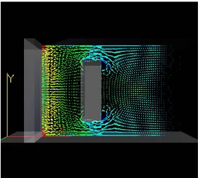
Flow past rectangular obstruction

Figure 1.1: Flow past obstruction initial wake formation

Figure 1.1 shows the piston driven flow at a point shortly after the piston was impulsively started (from left to right). Flow separation at the corners of the obstruction are clearly evident. The figure also shows a leading pressure wave that has diffracted around the edges of the obstruction.

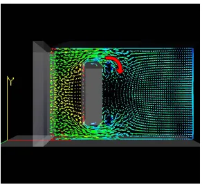
Figure 1.2: Wake development

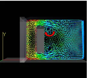
Figure 1.3: Further wake development with eddies

In all of these figures, separation at the sharp leading edge corners of the block can be observed. While it isn’t clear in these images, there exists a small region of re-circulating flow behind the separation points. Particles flow around these re-circulating regions and accelerate through the narrow gaps between the block and the channel walls.

Flow through narrow gap

Figure 1.4: Piston driven flow through gap

Figure 1.5: Formation of “cavities”

After gaining much more experience using SPH, and DPM, I now realize that these cavities must be the result of centrifugal acceleration as the particles’ velocities follow the curved path in the wake eddies. That centripetal acceleration tends to pull the particle away from the center of rotation resulting in the cavity. However, what we really have is a void in the flow simulation where there is no computational capacity since the computational nodes have evacuated the region. Therefore, we’re unable to capture any flow information in these void spaces. This turns out to be a significant drawback of Lagrangian methods since certain flow characteristics of interest can result in the loss of resolution in the regions where resolution is most needed or desired. As you’ll see later, the DPM is a hybrid method in that it can perform as either a Lagrangian method or an Eulerian method allowing one to choose the approach best suited for the problem at hand.

Breaking dam

The following series of images (Figures 1.6, 1.7, 1.8, and 1.9) show a few frames from a breaking dam simulation using this present program. The color scale represents particle speed with red representing higher speeds and blue representing low or zero speed.

Figure 1.6: Initial particle configuration and start of motion

Figure 1.7 shows two time instances where the falling column has reached the opposite end of the container and begins to splash up the container wall.

Figure 1.7: Fluid impacting container wall

Figure 1.8: Fluid breaking back on itself

Figure 1.9: Initial secondary splash created by fluid-fluid impact

near boundaries facilitate improved simulations that are more accurate, stable, and that do not require prohibitively small time steps.

Methods for Dealing with Cavity Flow

Aside from the motivation provided from my initial tests using SPH, cavity flows in and of themselves are an interesting phenomenon worthy of study. Cavitation is prevalent in a wide variety of fluid flow problems; everything from industrial process flows, to pumps and propellers, to high speed underwater projectiles, to space craft engines, to artificial heart pumps and valves involves cavitating flow. The phenomenon is widespread, and relevant. It’s understanding is critical in applications where its detrimental effects must be mitigated or controlled. Cavitation, especially at high Reynolds numbers where turbulence is involved, is a complex phenomenon and is difficult to model accurately. Attempts to model cavitating flow have been undertaken for over one hundred years [32].

Classical methods for modeling fully developed cavity flow include potential flow methods that assume inviscid, irrotational and incompressible flow.[32] [34] For flow outside the thin boundary layer and for problems with well defined, easily predictable cavity detachment points these models yield reasonable results. They tend to break down when the detachment point is not well defined. In some problems cavitation does not occur on the body or at a sharp detachment point but instead occurs in the wake (in shed vortices for example).[36][37] Even for cleanly detached cavity flow, classical methods have difficulty modeling cavity closure as this area consists of turbulent flow patterns not easily handled using distributions of sources or boundary elements. [32]

Attempts to resolve cavity closure using potential flow methods have led to various so-called closure models. These models include simple models where the cavity is assumed to close at a neat, well defined point as well as more complicated models where the cavity closure forms a re-entrant jet. The single point closure approach is clearly unrealistic, and even the re-entrant jet model represents far more ordered flow patterns than what actually exist.[32]

vorticity generation) in closure regions, and compressibility of vapor or non-condensable gas and of the multi-phase fluid mixture.[41][52][54]

The authors of [40] discuss various computation approaches for dealing with cavitating flows. These methods include Eulerian, Lagrangian, and hybrid methods. The authors recognize, and this is backed up by other authors, that multiphase flow is very complex and computational methods still are not well developed to deal with many of the previously mentioned complexities inherent in cavitating flow.

Many modern methods use single fluid models where volume fractions and mixture density is evolved using transport equations, while other methods use multi-fluid models with transport equations suited to each component of the flow. In most cases, the methods employ some sort of mesh or computational grid. Such grids always present problems where sharp interfaces exist and resolution may be lost. Therefore many methods attempt to employ some form of interface tracking algorithm such as level sets or one-way coupled Lagrangian methods. In these cases, usually the non-cavitating velocity field is computed with a method such as a RANS code and then fronts (e.g., using implicit surfaces) or particles are evolved subject to the previously computed velocity field [53]. These methods ignore the effects of cavities on the velocity field.

Several methods, [48], [49] and [51] for example, incorporate bubble or non-condensable gases along with vaporization models and track bubble evolution using some form of the Rayleigh-Plesset equation. [51] discusses several limitations of this approach including numerical instability issues and inaccuracies when liquid-vapor density ratios are large (which often occurs in cavitating flow) and when pressure differences are large between inflow and outflow points in the computational domain. Further, results are reported to be very sensitive to initial, specified conditions and require the use of tuned relaxation factors to improve results.

occurring when the fluid pressure drops below the liquid vapor pressure leads to inaccurate predictions since effects of nuclei are ignored. Carefully controlled experiments indicate that liquids can sustain large tensions even when the pressure falls well below the vapor pressure without resulting in cavitation events. Moreover, flows with realistic nuclei densities have been shown experimentally to result in cavitation inception even when the fluid pressure has not fallen below the vapor pressure of the liquid. These results highlight the importance of cavitation nuclei on cavitation inception. Attempts have been made to model the cavitation nuclei in numerical simulations. However, difficulties have been encountered due to the different scales involved and the fact that many methods use a continuum model which is inherently inaccurate for simulating discrete nuclei and sharp free-surface like interfaces in cavitating flows. In general, the jury is still out as to which method/model best captures complicated cavitating flow phenomenon.

Several researchers [16] [30] have used SPH to model multi-phase flow in the context of astrophysics simulations, e.g. for such things as star formation. In these cases, they deal with compressible gases along with other physics such heat transfer, magnetic effects and gravity. More down to earth problems such as air entrainment in breaking waves [25] [31] [39], e.g., around ship bows or ocean waves breaking near shore, have been investigated using multi-fluid versions of SPH. In these latter cases, focus is on modeling two fluids such as air and water and not the multi-phase, with phase transition, phenomenon of cavitation. Some researchers [1] [2] have applied SPH to simulate high pressure die casting processes involving liquid to solid phase transitions. I feel that valuable techniques can be borrowed from all of these fields and applied to the simulation of cavitating flow problems.

At the start of this research I held the view that SPH, or a derivative thereof, offered several compelling advantages for application to cavitating flow problems; namely:

• The Lagrangian nature of SPH eliminates troublesome convective acceleration terms

from the momentum equations

• SPH along with recent improvements for front tracking can handle sharp density

• SPH readily facilitates incorporation of different physics/models, such as surface tension, chemical reactions, thermodynamics, etc.

• SPH can handle multiple fluids

• SPH naturally models compressible fluids

• Physical viscosity can be modeled in SPH

• Turbulence can be treated in SPH

• SPH models buoyancy

• SPH, due to its Lagrangian nature instead of a continuum approach, naturally handles

particles and sharp interfaces facilitating the modeling of cavitation nuclei and free-surfaces

In general, I still hold this view with the exception of the Lagrangian nature mentioned above. My work has revealed that for cavity flows, at least the problem I studied, are better dealt with using an Eulerian approach. Fortunately, as mentioned earlier, the DPM works either way as will be discussed in greater detail later.

C h a p t e r 2

THE DISTRIBUTED POINTS METHOD (DPM)

The Distributed Points Method (DPM) is a meshless method for numerically solving differential equations, specifically, the Navier-Stokes equations in this study. The DPM is essentially a particle method similar to and inspired by the method of Smoothed Particle Hydrodynamics. Particle methods are attractive to use in the numerical modeling of complex fluid flows because the particles, which are computational nodes, are disconnected in the sense that there’s no mesh or connectivity scheme to constrain node position. This means that for complex flows, such as free surface flows, there’s no need to worry about issues such as mesh entanglement that cause serious problems in meshed based methods.

Splashing, fluid breakup and coalescence are easily handled by particle methods without the need for elaborate mesh management and re-meshing schemes. Moreover, considerable time is spent setting up and tuning meshes in meshed-based methods, whereas, particles are relatively easy to set up for meshless methods. That said, there are some problems that present difficulties for particle methods like SPH. For example, problems involving high density ratios generally require some form of particle redistribution intermittently during a simulation to ensure stability and reduce errors that occur when particles become disorganized. Density ratios on the order of 1000 to 1 are required for cavitating flow problems. Such density ratios are quite steep and care has been taken during development of the DPM to ensure the method can handle these density ratios.

An ability to handle high density ratios is just one of the goals I had in mind when developing the DPM. At the onset of this research, I wanted to develop a method that:

1. was meshless and could be used in either a Lagrangian or an Eulerian fashion.

2. could handle large density ratios, specifically density ratios of 1000-to-1.

4. would be easy to extend to handle multiphase flow with phase transition.

5. would be scalable in terms of having the ability to relatively easily add more physics to the governing equations.

6. would be straightforward conceptually and relatively easy to program.

7. would be relatively easy to parallelize.

My rationale for the first goal listed is due to a recognition of the demonstrated flexibility and adeptness of SPH – a Lagrangian method – to handle a wide variety of complex flow problems. On the other hand, it’s well known that specification and enforcement of boundary conditions is more straightforward in Eulerian methods. Further, Eulerian methods don’t suffer from the issue of particles evacuating a specific location in the fluid domain due to dynamic action.

Large density ratios are present in the cavitation problems I’m interested in investigating; therefore, having the ability to cope with density ratios on the order of 1000-to-1 as stated in the second goal above is a requirement.

Regarding the third stated goal, while the SPH formulation for computing gradients is attractive in that gradients are simply analytically derived given the kernel approximation, the simplification made in SPH results in errors when applied near boundaries. There are several approaches for reducing the error in SPH, however, they add complexity to the overall formulation and implementation.

One of SPH’s attractive features is that it’s relatively easy to implement a wide variety of state equations describing the pressure-density relationship and to add new physics to the governing equations. Given my desire to adapt the new method to multiphase flow I wanted to retain this characteristic. Goals four and five stem from this desire.

popular in the first place, and that is its simplicity both conceptually and in implementation. As stated in goal six, I wanted to preserve a fundamental simplicity in the method I developed not only for selfish reasons as it would make my work easier but also to make the method readily accessible to students for pedagogical use and experimentation.

Finally, as stated in goal seven, I knew that leveraging computing clusters would be a requirement for performing complex, high resolution simulations. Therefore, I wanted a method, like SPH, that was relatively straightforward to parallelize.

Having already researched many state of the art computational fluid dynamics methods during my coursework, I knew that SPH was the method of choice for my purposes with the exception of the problems I’ve already discussed. Therefore, with SPH as a model and inspiration I began development of the new method by starting with the governing equations and figuring out the most straightforward way of computing the required derivatives of field values, after all, computation of these derivatives is the heart of any numerical scheme. My first decision was to retain the meshless nature of SPH along with its interpolation concept. However, I wanted to avoid transforming the governing equations and instead compute the required derivatives applying them directly in the original form of the governing equations.

After much trial and error and several failures, the solution I found was to develop shape functions representing the field values that required differentiation and to differentiate those shape functions analytically. In order to fit these shape functions to the underlying field values, I adopted the method of least-squares along with an SPH-like weighting function and nearest neighbor scheme. Basically, field values at any given particle are the weighted averages of values at that particle and its nearest neighbors. Further, the particles have finite support in that only neighbors in the immediate vicinity of any given particle contribute to the weighted average. This is essentially the SPH interpolation scheme. However, unlike SPH I don’t use the derivative of the weighting function to approximate derivatives of field values; instead, I fit a shape function and differentiate the shape function. This approach is further discussed later in this chapter.

compressibility approach is somewhat more straightforward to implement, plus I wanted the flexibility to deviate from a purely incompressible flow solver since I anticipated compressibility being a factor in vapor filled cavity flows.

Governing Equations

The governing equations adopted in the DPM are the incompressible Navier-Stokes equations,

y x g y v x v y P Dt v D g y u x u x P Dt u D + ⎟⎟ ⎠ ⎞ ⎜⎜ ⎝ ⎛ ∂ ∂ + ∂ ∂ + ∂ ∂ − = + ⎟⎟ ⎠ ⎞ ⎜⎜ ⎝ ⎛ ∂ ∂ + ∂ ∂ + ∂ ∂ − = 2 2 2 2 2 2 2 2 ) ( ) ( μ ρ μ ρ

All of the work carried out as part of this research has been in 2D; therefore, the above equations are the 2D Navier-Stokes equations. Extension of the method to 3D would involve adding another momentum conservation equation for the z-coordinate direction and selection of a suitable three dimensional shape function (to be discussed later). In these momentum conservation equations,

ρ represents fluid density, u the fluid velocity in the x-direction, v the fluid velocity in the y-direction, P

the pressure, μ the viscosity, gx is a body force term in the x-direction, and gy is a body force in the

y-direction.

As in SPH the DPM uses an artificial compressibility approach to approximate incompressible flow and adopts the following form of the continuity equation,

⎟⎟ ⎠ ⎞ ⎜⎜ ⎝ ⎛ ∂ ∂ + ∂ ∂ + ⎟⎟ ⎠ ⎞ ⎜⎜ ⎝ ⎛ ∂ ∂ + ∂ ∂ − = y v x u y v x u dt

dρ ρ ρ _ρ

So far these three equations – two momentum conservation equations and the continuity

equation – represent three equations with four unknowns u, v, ρ, and P. To close this equation system a suitable state equation relating pressure to density is introduced, namely,

Here, c is an artificial sound speed used to enforce incompressibility and γ is the specific heat ratio of the fluid (usually taken as 7 though in the phase change state equation discussed later in Chapter 5 it may differ from 7). This state equation is a standard barotropic state equation where pressure is an explicit function of density only. Temperature does not appear in this state equation although it certainly could in which case we would require an additional energy conservation equation to close the system. Some implementations of SPH take this approach when applied to problems where heat transfer is a significant part of the problem. I’ve ignored effects of temperature so far in this study. The state equation shown here is for single phase fluids such as water. Later in Chapter 5, I present a multiphase state equation developed for application of the DPM to cavitation.

As in SPH methods, DPM requires a suitable artificial sound speed, c, in order to approximate incompressible flow. The rule of thumb in SPH methods is that the resulting artificial Mach number should be less than or equal to 0.1 and I’ve adopted the same standard here; however, as part of a systematic sensitivity study to be discussed later I do vary the Mach number (see Chapter 4).

The momentum equations, shown earlier, are written using the standard substantial derivative operator. In the DPM, the momentum equations can be used in either Eulerian form, with convection terms, or Lagrangian form without convection terms. Expanding the substantial derivative term in the momentum conservation equations reveals the convective acceleration terms and the Eulerian form of these equations are thus as follows,

y x g y v x v y P y v v x v u dt dv g y u x u x P y u v x u u dt du + ⎟⎟ ⎠ ⎞ ⎜⎜ ⎝ ⎛ ∂ ∂ + ∂ ∂ + ∂ ∂ − = ⎟⎟ ⎠ ⎞ ⎜⎜ ⎝ ⎛ ∂ ∂ + ∂ ∂ + + ⎟⎟ ⎠ ⎞ ⎜⎜ ⎝ ⎛ ∂ ∂ + ∂ ∂ + ∂ ∂ − = ⎟⎟ ⎠ ⎞ ⎜⎜ ⎝ ⎛ ∂ ∂ + ∂ ∂ + 2 2 2 2 2 2 2 2 μ ρ μ ρ

Figure 2.1: Illustration of Eulerian Approach

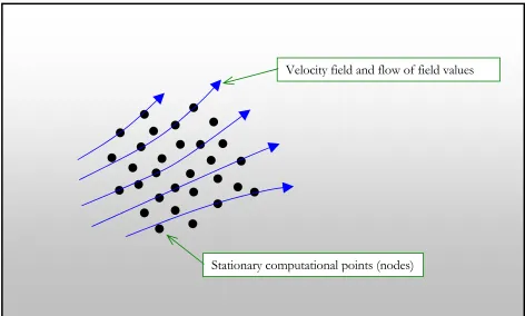
In the Lagrangian form there are no convection terms to deal with, which means that fluid properties will not be advected throughout the flow field as in the Eulerian case. However, in the Lagrangian case, the computational points themselves are advected in an manner similar to that seen in the SPH method. Figure 2.2 illustrates this concept.

Stationary computational points (nodes)

Figure 2.2: Illustration of Lagrangian Approach

The Lagrangian form of the momentum equations are simply,

y x g y v x v y P dt dv g y u x u x P dt du + ⎟⎟ ⎠ ⎞ ⎜⎜ ⎝ ⎛ ∂ ∂ + ∂ ∂ + ∂ ∂ − = + ⎟⎟ ⎠ ⎞ ⎜⎜ ⎝ ⎛ ∂ ∂ + ∂ ∂ + ∂ ∂ − = 2 2 2 2 2 2 2 2 μ ρ μ ρ

When the DPM uses this form, the points distributed throughout the fluid domain move with the fluid carrying fluid properties along with them. The points move by virtue of the velocity field they themselves represent and numerically it’s a simple matter of integrating the velocity field to compute displacements for each point in the fluid domain.

Both the Lagrangian and Eulerian approaches have been used in this research and both have their advantages and disadvantages. For example, inflow and outflow boundary conditions are easier to handle using an Eulerian approach; however, the Lagrangian approach eliminates the need to deal

Computational points (nodes) flow with fluid carrying fluid properties with them. Hatched circles represent node locations at time t while black circles represent new node locations at time t+dt.

with convective terms altogether. The DPM is flexible enough to handle both approaches affording options when modeling certain flow types. For example, free surface flows where splashing is important may be better handled using the Lagrangian approach, whereas the 2D cylinder flow problems discussed later in Chapter 4 are better handled using an Eulerian approach.

In the distributed points method, the governing fluid equations are not transformed for some discretization scheme but instead are used directly as shown. This is achieved through the use of suitable shape functions that represent fluid field values such as velocity and direct analytic differentiation of those shape functions. The shape functions are discussed next.

Gradient Computation

A key feature of the DPM is the combination of an interpolating kernel in the sense of SPH with least squares approximations for field values in order to compute spatial derivatives in the governing equations.

In SPH, interpolation kernels are used to derive an approximation of the gradient of field values in terms of the gradient of the interpolation kernel. This is a well known approximation in the SPH literature. It is also well known that such an approximation for gradients possesses several deficiencies when computing gradients near boundaries. In the DPM we use interpolation kernels in a somewhat different manner.

Given a set of dispersed points with spatial coordinates and associated field values, we can interpolate the field value of interest at any coordinate using an interpolation kernel as follows,

( )

_∫

( ) (

)

A _{i k i}, _k

where W is a weight function that gives more weight to points, x_k, that are closer to the point

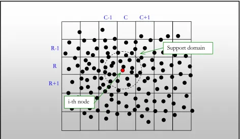
Figure 2.3: Illustration of weighted interpolation

It should be noted that A(x) and W(x) are functions of the vector coordinates of each node

such that in two dimensions A is a function of both x and y, as is W. In the case of a discrete set of unconnected points we have,

( )

_∑

( ) (

)

A ,

over all k points.

This is the same interpolation formula forming the basis of SPH. In practice, this formula is essentially a weighted average of field quantities surrounding the point of interest. The important element to emphasize here is that values closer to the point of interest are given more importance – more weight – than values further from the point of interest.

In DPM, these weights are also used in another way. Specifically, the DPM uses a weighted least squares method to derive coefficients for shape functions representing field values where these

Only neighbors within a node’s circle of influence contribute to the interpolation

i-th node

k-th nodes

shape functions are then differentiated analytically to compute spatial derivatives. This is where DPM starts to differ from SPH. As discussed earlier, SPH uses the gradient of the weight function to approximate derivatives and the governing equations are transformed to accommodate this approximation. Since in the DPM derivatives are computed for analytic shape functions directly representing field values, we can apply the governing equations directly without transformation.

In the DPM we assume that field values at any point can be approximated by a function of the form,

∑

f ϕ

The an coefficients are determined in the usual least squares manner by minimization of the

weighted residual,

(

) (

)

[

_∑

]

2 min

considering all k points in the support domain of the point, i, under consideration. F is the actual field

value at the point considered and f is the approximated field value. Depending on the form of the

shape function, there are several approaches that can be taken to find the an coefficients. For example,

if the field values are locally approximated by a linear function (for two-dimensional problems where field values are functions of the x- and y-coordinates),

y a x a a

f = o + 1 + 2

then the normal equations can be derived relatively easily and the coefficients solved for directly. For other functions, like the bi-quadratic function (again for two-dimensional problems),

2 5 4

2 3 2 1

0 a x a y a x a xy a y a

f = + + + + +

functions more stable and better capable of handling steep gradients, such as density gradients that appear in cavitating flow. Moreover, second derivatives can be computed easily for diffusive terms in the governing equations rather than using repeated linear approximations which result in greater approximation error.

Once the least squares coefficients have been determined for all field values – pressure, velocity, and density – at each node, spatial derivatives are computed by direct differentiation of the shape function. For example, first derivatives in x are,

y a x a a x f

4 3 1 +2 + =

∂ ∂

With proper centering of all coordinates about the x_i coordinate while performing the

weighted least squares fit all terms involving x or y drop out, yielding simply,

1 a x f

= ∂ ∂

Similarly, second derivatives reduce to the form,

3 2 2

2a x

f = ∂ ∂

Least Squares Fit

Before settling on using the bi-quadratic shape function, with a direct solution to the normal equations, I tried several different approaches. These approaches include:

1. Use standard least-squares algorithms to fit bi-quadratic shape functions.

2. Derive the bi-quadratic normal equations and solve directly.

3. Derive a plane equation shape function for use when computing pressure and density

gradients.

4. Derive a two-part shape function using quadratic polynomials.

5. Derive a two-part shape function using linear polynomials for computing pressure and density

gradients.

My primary incentive for trying these five different approaches was to find the approach that yielded the most efficient computation time. As it turns out the best approach, and the one used for the simulations presented herein, is a combination of two of the above approaches. Bi-quadratic shape functions solved in closed form were used for velocity gradients where second derivatives are required. Plane equation shape functions solved in closed form were used for density and pressure gradients where only first derivatives are required. Each approach is discussed in greater detail in the following paragraphs.

Standard Least Squares Algorithm

would be to solve the least squares normal equations by hand, analytically, and program the solutions for the fit coefficients avoiding any sort of runtime matrix inversion. This approach is discussed next.

Bi-quadratic Shape Function Solved Directly

Applying the method of least squares to find the six coefficients of the bi-quadratic shape function shown earlier requires finding the simultaneous solution to the six normal equations representing the minimization of weighted, squared residuals. The normal equations for the bi-quadratic shape function are found by taking the derivative of the sum of weighted, squared residuals expression shown earlier for each of the six coefficients, an, and equating the resulting expressions to

zero. For example, let

(

) (

)

∑

= F_k f_k W x_i x_k

q 2

which is the expression we want to minimize. Fk represents the actual field value at the kth nearest

neighbor to node i under consideration, while fk represents the approximated field value at the kth

nearest neighbor using the bi-quadratic shape function. W represents the weight value for the kth

nearest neighbor as a function of the distance from the kth _{neighbor to the i}th _{node under}

consideration. Letting z be the value of Fk, w be the weight for kth neighbor, and substituting the

bi-quadratic shape function yields the following expression for q,

(

)

(

)

[

]

∑

= z a a x a y a x a xy a y w

q _{0 1 2 3} 2 _{4 5} 2 2

Here the summation is over n nearest neighbors to node i, including node i, and the k subscripts have been dropped for simplicity.

To get the first of the six normal equations you take the partial derivative of q with respect to the first coefficient, a0 as follows,

Setting the derivative of q with respect to a0 equal to zero, rearranging, and distributing the summation

yields the following normal equation,

∑

∑

∑

∑

∑

∑

∑

5 4 2 3 2 1

0 w a xw a yw a wx a xyw a wy

a zw

Following a similar procedure for each of the five remaining an coefficients yields five additional

normal equations as follows,

∑

∑

∑

∑

∑

∑

∑

∑

∑

∑

∑

∑

∑

∑

∑

∑

∑

∑

∑

∑

∑

∑

∑

∑

∑

∑

∑

∑

∑

∑

∑

∑

∑

∑

∑

(

)

(

)

(

)

(

)

(

)

The β terms in these equations are,

57 65 67 55 67 56 65 66 55 66 θ θ θ θ β θ θ θ θ β − = − =

The θ terms are,

7 , 6 , 5 6 , 5 , 4 4 44 = = − = k j for k j jk

jk γ γ γ γ

θ

The γ terms in these equations are,

7 , 6 , 5 , 4 6 , 5 , 4 , 3 3 33 = = − = k j for k j jk

jk φ φ φ φ

γ

C I D T B A N = = = = = = = 06 05 04 03 02 01 00 φ φ φ φ φ φ φ AC ON AI FN AD EN AT HN CB DN AA TN − = − = − = − = − = − = = 16 15 14 13 12 11 10 0 φ φ φ φ φ φ φ

(

)(

) (

)(

)

(

)(

) (

)(

)

(

)(

) (

)(

)

(

)(

) (

)(

)

(

)(

) (

)(

)

(

)(

) (

)(

)

(

)(

) (

)(

)

(

)(

) (

)(

)

(

)(

) (

)(

)

(

)(

) (

)(

)

(

)(

) (

)(

)

(

)(

) (

)(

)

(

)(

) (

)(

)

(

)(

) (

)(

)

(

)(

) (

)(

)

(

)(

) (

)(

)

(

)(

) (

)(

)

(

)(

) (

)(

)

(

)(

) (

)(

)

Finally, the coefficients appearing on the right sides of all the φ terms are,

Using these equations to find the unknown coefficients is dramatically faster computationally than using the standard least squares algorithms discussed earlier. While these equations may look cumbersome they are relatively straightforward to program.

As discussed earlier, with proper centering of coordinates, partial derivatives of field values approximated with the bi-quadratic function are simply:

1 a x f ₌ ∂ ∂

3 2 2

2a x

f ₌ ∂ ∂

2 a y f

= ∂ ∂

5 2 2

2a y

f ₌ ∂ ∂

This formulation is useful for approximating the velocity field where first and second derivatives are required as seen in the governing Navier-Stokes equations. For pressure and density, however, second derivatives are not required and a simpler formulation may be used.

Plane Equation Shape Function

The plane equation,

y a x a a

f = o + 1 + 2

A C M A

C B AM

BG P

A BD H N

A B F M

− −

= − =

− =

2 2 2

Now partial derivatives reduce to,

1 a x f

= ∂ ∂

2 a y f ₌ ∂ ∂

In principle, the bi-quadratic function could also be used to approximate pressure and density derivatives; however, it involves more computations making the plane equation approach more efficient. Moreover, numerical tests using the bi-quadric equation to approximate pressure resulted in relatively noisy pressure fields.

Two-part Polynomial Shape Functions

Figure 2.4: Two-part shape functions

For example, referring to Figure 2.4, we’re interested in the derivatives of the field values, u_i, at the point represented by node i. All k nodes store the field value, uk, at their respective locations. If

you graph u as a function with respect to position x and y, you’d get a surface. We’re interested in the derivatives of ui with respect to x and ui with respect to y. Graphically speaking we can compress all

nodal values onto the u-x plane around the ith _{point of interest. We further compute the relative}

coordinates of each kth _{point with respect to the i}th _{point. The resulting plot shows how u changes}

with respect to x. This two dimensional graph can then be fit with a function using a weighted least

squares method as discussed herein. Now, the weights used to weigh the contributions of the k point

values must be a function of distance in the x, y plane from the kth _{point to the i}th _point.

Repeating this process and compressing the points onto the u-y plane will result in another

graph for which we can fit another function. The first function can be differentiated to approximate the derivative of u with respect to x, while the later function can be differentiated to approximate the derivative of u with respect to y.

Support domain

i-th node

k-th nodes

|u|

|u|

x y y

x

Projection onto u-y plane

Using this approach for the velocity field would require at least a quadratic interpolation function allowing the computation of second derivatives. For pressure and density fields, linear shape functions can be used.

This approach generally works fairly well. Numerical tests show relatively good computation efficiency and the approach is straightforward to program for two dimensional flow simulations. The drawback with this approach is that it’s more cumbersome to implement for three dimensional flow simulations. Given my desire to extend this method to three dimensional problems, I’ve opted to retain the bi-quadratic and plane equation shape function approaches discussed earlier.

Weighting Function

The least squares approximation just described relies on a weighted least squares approach where nodes further from the given node under consideration, the ith _{node, are given less importance –}

weight – while performing the least squares calculations. This approach mimics physical reality in that activity at a point in the fluid is less and less influenced by activities further and further away from that point.

Chapter 1 describes how weighting functions are used in SPH. The most common weight function used in SPH is the cubic spline approximation to a Gaussian weight function as shown in Chapter 1. Many different forms of the weight function may be used; however, SPH does require the weight function to possess certain characteristics, namely: that the function is normalized; that it is differentiable, analytically, to the degree required in the particular SPH formulation; that it has a smooth second derivative; that the function has compact support; that the function is even and positive; that the function approaches the Dirac delta function as the smoothing length goes to zero.[24]