The Effect of Exchange Rate, Oil Prices and Global Inflation Shocks on Macroeconomic Variables for the Iranian Economy in the form of a DSGE Model

The Effect of Exchange Rate, Oil Prices and Global

Inflation Shocks on Macroeconomic Variables for the

Iranian Economy in the form of a DSGE Model

Sajad Boroumand2_{, Teimour Mohammadi*}3_, Jamshid Pajooyan4_{, Abbas Memarnejad}5

Accepted: 2019, February 2 Received: 2018, November 28

Abstract

he world economy has experienced a bulk of positive and negative shocks in crude oil prices and exchange rates over the years, and that global inflation has undergone some changes. Such shocks have affected the macroeconomic variables in the countries of the world and have challenged the economies of these countries, and have led them to take different measures to protect themselves against the devastative effects of these shocks. Accordingly, the main objective of the current study was to analyze the dynamic effects of three external shocks (global oil price shock, euro / dollar exchange rate shock and global inflation shock) as well as to investigate the appropriate monetary policy strategy for the Iranian economy, given the structural characteristics and patterns of external shocks. In so doing, we analyzed the responses of external responses to external shocks according to alternative monetary rules, including Headline Inflation Targeting (IT), Core Inflation Targeting (CIT), and Exchange Rate (ER) rule. Therefore, in this research, the goal was to determine the monetary policy rule to minimize both macroeconomic fluctuations and keep inflation at a low level. Furthermore, we strived to answer the question that whether the inflation criterion in Iran should be headline inflation, core inflation or exchange rate. To answer this question, using the DYNARE software, we estimated a multiplicative New Keynesian Dynamic Stochastic General Equilibrium model based on the characteristics of Iranian economy. Our primary finding showed that core inflation rule was the best monetary rule for stabilizing both macroeconomics and inflation.

Keywords: Monetary Policy, Core Inflation, DSGE Model. JEL Classification: E52, E31, D58.

1. Introduction

The formulation of socio-economic development programs and the

1. The article is extracted from PhD dissertation of Sajad Boroumand, Science and Research branch, Islamic Azad University, Tehran, Iran.

2. Department of Economic, Science and Research branch, Islamic Azad University, Tehran, Iran (borus_181@iauksh.ac.ir).

3. Faculty of Economics, University of Allameh Tabatabae’i, Tehran, Iran (Corresponding Author: mohammadi@atu.ac.ir).

4. Faculty of Economics, University of Allameh Tabatabae’i, Tehran, Iran (j_pajooyan@atu.ac.ir). 5. Department of Economics, Science and Research Branch, Islamic Azad University, Tehran, Iran (ab_memar@srbiau.ac.ir).

establishment of the country's annual budgets and the design of appropriate policies for maintaining economic stability and equilibrium requires the identification, examination, and accurate prediction of the impact and volatility of oil price, exchange rate, and global inflation on macroeconomic variables, so that planners can adopt the right policies in the event of oil and exchange fluctuations as well as global inflation, and reduce its impact on macro variables to the minimum. Therefore, the argumentation of the impact of various shocks on Iran's macroeconomic variables, as an oil-rich country and an oil exporter, seems quintessential. Therefore, economic policymakers have sought to find the best monetary policy model that, in addition to stabilizing macroeconomic variables, could reach inflation rate to its lowest level.

In this paper, we focused our attention on Iran as a small open economy, which exports oil and estimated a Dynamic Stochastic General Equilibrium (DSGE) model with a new Keynesian approach for Iran's economy through which we investigated the dynamic effects of three external shocks (oil prices, exchange rates, and foreign inflation) and tested the appropriate monetary policy rule. To do this, we developed a multi dynamic stochastic general equilibrium (MDSGE) model with real and nominal inflexibility. The goal was to firstly compare the importance of each shock as a source of fluctuations in Iran's economy and, secondly, to define an appropriate monetary rule that protects the economy against the effects of these shocks.

imported sectors; this allows monetary policy to play a role in our model. In fact, this assumption is very important for examining the role of monetary policy in a DSGE model. We have considered three alternative monetary policy principles: a fixed exchange rate rule, an inflation targeting rule, as well as a core inflation targeting rule. We adopted these rules for two main reasons: (1) they describe the implementation of monetary policy in a large number of emerging market economies; and (2) in the oil export economy, the presence of a petroleum component in the CPI inflation index raises the question of whether the inflation criterion in Iran should be headline or core. In other words, is monetary policy in Iran reacting to headline inflation or to core inflation?

The rest of the article is organized as follows: in Section 2, the related literature and studies in this regard are reviewed. In Section 3, the details of the model is scrutinized. Section 4 discusses calibration parameters, data, and priorities. Section 5 presents the estimation results. Section 6 measures the effect of external shocks under the rules of alternative monetary policy. Furthermore, Section 7 deals with the conclusions.

2. Review of the Related Literature 2.1 New Keynesian Model

The new Keynesian term was first introduced in 1982 in the book Macro economy by Bade and Parkin (1982). The new Keynesian macro economy is the modern school of thought, developed on the Keynesian idea, and is, in fact, a response to the critique of the new classics. In fact, new Keynesian is not a new reinterpretation of Keynes's theory, but rather a new embodiment of the idea that it uses some of the key elements of new and monetarist classics, and this is to a degree that Mankiw believes that new Keynesian macroeconomics is a kind of new monetarism school.

The initial and important difference between the new classical school and the new Keynesian school lies in the moderation rate of wage and prices; the new classical theory is based on the flexibility of wages and prices, so that prices are quickly adjusted in order to meet

the market clearing price But on the opposite side, new Keynesian

short-term economic fluctuations, and thus develop patterns that are along with wage and price stickiness. Based on wage and price stickiness, the new Keynesian theory seeks to answer the question of, firstly, why there is unemployment, and secondly, why monetary policy has real effects on the level of economic activity.

In the 1990s, the controversy between the new classics and new Keynesian highlighted the need for a new mix of economists to identify the best way to explain short-term economic fluctuations as well as the role of monetary and financial policies. The purpose of this combination was to combine the strengths of rival theories in order to identify a coherent process and structure for a better analysis of economic

fluctuations.This integration was developed in such a way that the new

classical model, tools for modeling the behavior of households and enterprises over time, was based on the optimization of their target function, and the new Keynesian model assumed that the wage was sticky to show why monetary policy has an impact on employment and

production in the short term. The most common way of modeling this

assumption is to consider enterprises in a monopolistic competition structure, in which both the enterprises have the ability to determine prices, and because of the existence of competitive space, price changes will occur periodically.

The main focus of this new integration is based on the idea that economy is a dynamic general equilibrium system which, in the short term, has deviated from the level of resource allocation for some reason, such as price stickiness and some market imperfections. This feature provides a good place to analyze monetary and financial policy.

2.2 Theoretical Fundamentals of the New Keynesian Model

As noted in the previous section, in the new integrative approach, economy is assumed a dynamic stochastic general equilibrium system, which is associated with nominal adhesions such as price stickiness. In a dynamic stochastic general equilibrium system, segregation of economic sectors is possible in two ways:

among this type of modeling, in which the government does not have

any role an economic balance.

In the second case, taking into account the role of the government in reallocating resources and its effects on economic dynamics, the model consists of three sections of the household, enterprise, and economic transition that usually involves the government and the central bank. The new Keynesian method falls into this category because, despite the assumption of price stickiness and market failure, monetary and fiscal policies have the potential to affect the real economic equilibrium (at least in the short term).

Another distinction between the first and second modes is that the new classical model is a non-money economy, in which the exchange of goods and services is carried out without any intermediary (money), and there is no asset called money. However, in the analysis of the new Keynesians, which have a role for the government, the need for money in the model is necessary. In terms of money in the new Keynesian general equilibrium models, there are three general methods:

1. In the first mode, households are assumed to be desirable to maintain a real cash balance (Sidrauski, 1967). This method is known as money in utility function.

2- In the second case, money can be put into modeling in the form of speculative demand for money. Hence, one can do this in three methods:

- The first method is the concept of cash-in-advanced constraint, which was first introduced by Clower (1967). In this method, the role of money is defined as the intermediary of the exchange used for the purchase of consumer goods. In fact, in addition to budget constraints, the household will face a liquidity constraint, so that household expenditures should not exceed the level of money balance.

- Real resource costs: According to Brock (1974) and Brock and Lebaron (1990), transaction costs are assumed to be in the form of

real resources consumed in conversion process. Specifically, an

- Search theory and money as a medium of exchange: In this approach, the natural nature of money is introduced into modeling as a medium of exchange; for example, in Kiytaki and Wright (1993) model, exchange of goods is possible, but finding a product that makes the exchange possible is costly; however, the existence of an unpaid money can make the exchange possible (Tavakolyan, 2017).

According to the above, a random dynamic stochastic general equilibrium model based on the new Keynesian approach consists of three parts of the household, enterprise, and economic transition policy. According to the study and modeling, each of these three sections can include the various subdivisions. They will be referred to in the next section.

2.3 Previous Studies

Today, many central banks have introduced their monetary models in the form of DSGE models used in the New Keynesian School. For example, the central banks of England (Harrison et al., 2005), Canada (Murchison and Rennison, 2006), and even Chile and Peru (Castillo et al., 2008) use these models in their analysis and explain the behavior of their economies, and the effect of different policies is increasingly being examined in the form of DSGE models.

In the context of the research, there is a dearth of domestic research on the effects of external shocks on macroeconomic variables under alternative monetary policy rules. However, Faraji and Afshari (2014), in a nearly similar research, investigated the impact of oil prices and

monetary policies in Iran with the new Keynesian approach. In their

study, aiming at identifying an optimal monetary policy in the face of oil price shocks, a multi random dynamic equilibrium model emphasizing the optimization of the oil sector was addressed. In their paper, using the Bayesian approach, the impact of various monetary policy rules was examined.

3. The Model

The main framework of the DSGE model in this study inspired from the papers by Allegret and Benkhodja (2015), Ireland (2004), Dib et al. (2003), Leduc & Sill (2004), Medina & Soto (2006), Walsh (2003) as well as from some of the domestic articles such as Faraji and Afshari (2014) referred to in the literature review.

In this section, we simulate an oil export economy based on the characteristics of the Iranian economy. To do this, we assume that seven actors surround economy: domestic residents, oil companies, non-oil producers, imports of foreign intermediate goods, final goods producers, central banks, and government.

3.1 Households

Households gain utility from Ct and leisure (1-ht). Household preference is described by the following utility function:





0 t t

t t

h c U

E







 (1)

Where β represents the internal degradation factor (0 <β <1). We assume that u (.) is the momentary utility function, and is determined by the following equation:

 

u . ,

1 1

 

 

    ₍₂₎

where the preferential parameters γ and σ are strongl dfui

y positive. The first parameter, γ, is the inverse of inter-temporal substitution elasticity of consumption and second parameter, σ, represents the inverse of the labor supply wage elasticity. The utility function of the unit, u (.), is shown to be very concave, which strongly increases in Ct and decreases strongly in ht. We also assume that ht is defined by Cobb-Douglas technology as follows:

, , ,

o hn ho

t no t o

t h h

h   

Finally, households accumulate shares of ko, t and kno, t, which are used in oil and non-oil sectors for nominal leases Qo, t and Qno, t. Evolution of equity shares in each sector is equal to:









k_j,t1 1 _j,t  _j,t _{j j,t1}, _j,t ,  ,

(4)

Where δ is the standardized depreciation rate for all sectors (0 <δ <1) and Ψ_ (j, t) Ψj,t(kj,t+1, Kj,t), the adjusted capital cost paid by the

household and meets ψ_j′′(. ) < 0 and ψ_j(0) = 0, ψ_j′. The functional form Ψ_j (.)is as follows according to the study by Ireland (2003):



2 . _, 2 , 1 ,

, jt

t j t j j t j k k k              (5)

for j= o, no

The presence of investment adjustment cost shows that, outside of a steady state, the newly established capital price is different from the price of capital goods. In other words, Tobin’s Q is different from one (1). This form allows the total and final adjustment costs in a constant equilibrium equals zero. The cost and income presented above will result in the household budget being as follows:





_





_

t B e B Q k W h D

k R B e R B i c P , , , , , , 1

1  1  ,

 

for j= o,no

(6)

where P_ti_t = P_0,ti_0,t+ P_no,ti_no,t is the total investment in oil and non-oil sectors, respectively, and Pt is the consumption price index CPI) defined as follows: According to the initial value, the factor of the internal inhabitants {ct, k0,t+1, kn0,t+1Btd and Btf} to maximize the

solution leads to the following first order conditions:

t c ,t



  (7)





  (8)

1 1 1 1 2 1 , 1 , 1 , 2 , 1 , 1 , 2 , 1 , 2 , 1                                                          t j t j j t j t j t j j t j t j t j t j j t t t k k q k k k k k k E        (9) , 1 1 t t t t

t E R

          

 (10)

, 1 1 1 1              f t t t t t t f t t t

t _E s

k R s     (11)

qj,t=Q_Pj,t

t , πt+1 =

Pt+1

Pt , πt+1

f ₌ Pt+1f

P_tf , st = et P_tf

Pt and Ξt = ξt

P ̃_tf

P_tf represent

the real return of capital in each sector, CPI inflation, The world inflation rate is the real exchange rate of the Iranian dollar/rial and the real exchange rate of the euro / dollar, and Ptf وP̃tf represent the external

GDP moderator expressed in US dollars and euros. Also, λt represents the coefficient of budget multiplication in relation to the budget constraint. By combining equations (11) and (12), we obtain equation (13), which indicates UIP:

f t t t t t t t f t t s s k R R 1 1 1 1          (12)

external interest rate, the global inflation rate and the euro/dollar exchange rate, which is exogenous according to the AR (1) process, which is deduced follows:

  



 

 

f t R

f R

f

t f R f R f

R 1 log log _{1 ,}

log     

(13)

  



 

 

t f

f

t f f f

, 1

log log

1

log  _  _   _

(14)

 





 

 

log  _  _  _

(15)

Where Rf, πf and ξ represent the stable status values Rf_tand π_tfand ξ_t ، ρ_Rf وρ_πf وρ_ξ are auto-correlation coefficients and ε_Rf_,t ،ε_πf_,t وε_ξ,t are

unbounded and have a normal distribution with mean zero and standard deviations σσ_Rf وσ_πf وσ_ξ.

3.2 Oil Sector

To model the oil production, assume that the oil company is in full

competition and that the oil is exported with the international price P_o,tf ,

per dollar.

To maximize profit, Companies should solve the following maximization problem:





max _{, , , , , , ,}

, , _,

,

t t O t o t o t o t o t o f

t o t O h

k_{ot ot t} eP Y Q k W k P O

(16)

Where e_tP_0,tf Y_0,t is the income of the oil producer in terms of domestic

currency. To solve equation (17), companies must examine their function according to Cobb-Douglas technology as follows:

,

, , , ,

o o o

t t o t o t o t

o A k h O

Y    

(17)

represent, respectively, the capital share, k_o,t, labor, h_o,t, and the oil source, Ot, for oil production.

Thus, with respect to ee_t ،P_0,tf ،Q_0,t ،W_0,t and P_0,t, the oil producing

company, selects {k_o,t, h_o,t, O_t} to maximize equation (17) according to

equation (18).

First order conditions include:

o,t f

o,t o t o,t

o,t Y

q s p

k

 

(18)

o,t f

o,t o t o,t

o,t Y

w s p

k

 

(19)

o,t f

O,t o t o,t

t Y

p s p ,

O

 

(20)

where q_0,t= Q0,t

Pt , ω0,t =

W0,t

Pt , p0,t

f ₌P0,tf

Pt , po,t =

Po,t

Pt are the real return

on capital, real wages, real oil prices and the actual price of the oil

source. Equations (19) to (21) represent the demand for k_0,t, h_0,t and

O_t, respectively.

Finally, the changes in the external oil price, P_0,tf , oil source, Ot, and

technology shock, and A_0,t are determined by the following random

process:

 





 





log _o,f_{t P o}f _{P o}f_{,t 1 P}f_,t

o f

o f

o

P P

P    _ 

(21)

 





 





log Ao,t  A_o Ao A_o Ao,t1 A_o,t ₍₂₂₎

3.3 Non-oil Sector

In this section, we assume that non-oil producers operate under monopoly competition conditions. Based on this hypothesis, it is assumed that there is a chain of companies indexed by iε (0,1). Each

function:

 

   

 

, i A k i h iY i

Y no no Ino

t o t no t no t no t

no



 

 (23)

Where kn0,t, hn0,t and YYo,tI (i) are used by companies to produce

non-oil products. An0,t is a non-oil technology shock. This shock follows the

random process given below:

 





 





log Ano,t  Ano Ano Ano Ano,t1 Ano,t (24)

Also, αn0, βn0, θn0ϵ(0,1) and αn0+ βn0+ θn0 = 1. These

coefficients represent the capital share, ،k_n0,t, labor, h_n0,t, and refined

oil, and Y_o,tI (i), and are used as inputs in the production of non-oil products.

According to the time-dependent stochastic rule, each manufacturer has a constant probability of price change in each period. This

probability is determined by the relation (1-φno). Therefore, on average,

the price of non-oil products for the period _1−ϕ1

noremains unchanged.

As in the research (Ion, 1996), we assume that if non-oil product manufacturers are not able to change their price, they will index them for the CPI inflation rate according to the following rule:

𝑃_{𝑛𝑜,𝑡} = 𝜋𝑃_{𝑛𝑜.𝑡−1}

where π is the average long-term gross inflation rate. The problem of

maximizing the non-oil company can be written as follows:

 max    0







 



,

, _{, ,}

,



 

s not s t s t

s no i

P i h i

k_{not not not} E   D i P

(25)

The first-order conditions (derivation) of the maximization problem include

 

 

no,t no no,t

no,t

Y i

w mc ,

h i

 

 

, ,

, not

t no

t no no t

no mc

i k

i Y

q 

(27)

 

 

o,t no I no,t

o,t

Y i

p mc ,

Y i

  (28)

where q_n0,t=Q_Pn0,t

t , ωn0,t= Wn0,t

Pt , mcno,t= MCn0,t

Pt , po,t = Po,t

Pt are the real

return on capital, real wage, real final cost, and the real price of

domestic oil. The real final cost, mc_no,t, can be obtained by replacing

the obtained equations (28) - (30) in equation (25):

no no no no no no

no,t no,t o,t

no,t

no no no

q w p

mc

  

  



   (29)

The optimal pricing condition is obtained using the maximization equation (26):

 









s

s _s

0 no t s no,t s no,t s no,t s t k

s 0 k 1

no,t s

s s 1 1

0 no t s no,t s no,t s t k

s 0 k 1

E Y p mc

p i

1

E Y p



   

    

 





 

   

 

   



 

 _{ } 

  _{   }









3.4 Import Sector

The final product manufacturer, for its manufacturing needs, uses

imported combined goods, Y_I,t, purchased on an internal competitive

domestic market. To produce Y_I,t, the company uses distinct products,

YI,t(i), produced by a chain of domestic importers, represented by iε

(0,1) and one homogeneous intermediate goods produced abroad and

imported at world prices P_tf. Part of these imported goods is μ, in euro,

while the other part (1-μ) is calculated in dollars. Distinct products are

sold at prices P_I,t(i), which have been shown to be sticky in research

(Calove, 1983) and (Ion, 1996). Therefore, the importer faces a constant

probability in each period (1-φI), which changes its price, as in the

stable CPI inflation rate.

The importer's maximization problem can be written as follows:

 



 



 











 

~ 1 ,

~ max , _s s t I f s t t s t t I s s t s I i P i Y P e i P E t I       (31)

The nominal price index of total imports is evolving according to the following recursive form:

 









 

 

  



 _{  } 1

, 1 1 , 1 , ~

1 _{I nTt}

t I I t

I P P

P (32)

The division of equation (39) by Pt leads to the real price index of the following imports:

 





 

1 1 , 1 ,    _        _{ }      

 _{I It}

t t I I t I p p p (33)

3.5 Final Goods Producer

Assume that the final goods producer is operating under the full competition market and uses CES technology, which includes non-oil product, Ynot, which is manufactured in the country as well as imported goods YI,t

, 1 1 1 1

1   _

                _

no no I I

t Y Y

z (34)

Where τ> 0 represents the substitution elasticity between non-oil

product and imported goods, and xno and xI represent the share of

non-oil and imported products, respectively in the final product, where

x_no+ x_I = 1. To maximize its profit, the final goods producer chooses

the final product {Y_I,t, Y_no,t}.

no ,t

I,t no,t

I,t I t no t

t t

P P

Y z , and Y z ,

P P

 

   

  _{ }   _{ }

    ₍₃₅₎

Where Pt, PI, t and Pno,t are defined. Also note that the zero benefit condition implies that the price of the final product is equal to:





1 1

, 1

, 



 _

    

 _{I It no not}

t P P

P

(36)

Finally, it should be noted that the final product is divided between

total consumption and total investment so that: z_t = c_t+ i_0,t+ i_no,t.

3.6 Monetary Policy

In this research, we assume that the central bank modifies short-term

nominal interest rates, Rt, in response to the fluctuation of inflation rate

in the non-oil commodity sector (core inflation), πno,t, CPI inflation

(headline inflation), and exchange rate , St, given the Taylor type

monetary policy rule and according to the study by Faraji and Afshari (93), as follows:

1 + 𝑅𝑡

1 + 𝑅∗

⁄

= (1 + 𝑅𝑡1

1 + 𝑅∗

⁄ )𝑖 (𝑦𝑡

𝑦∗

⁄ )

(1−𝑖 )𝜇𝑦

(𝜋𝑛𝑜,𝑡

𝜋𝑛𝑜∗

⁄ )

(1−𝑖 )𝜇𝜋𝑛𝑜

(𝜋𝑡 𝜋∗ )

(1−𝑖 )𝜇𝜋

(𝑠𝑡 𝑠∗)

(1−𝑖 )𝜇𝑠

(37)

The policy coefficients μ_πno, μ_π and μ_𝑠measure the central bank's

response to the deviations π_no,t, π_tand s from the stable state levels.

When the central bank adopts a CPI inflation targeting system (IT

rule), μ_πno = μ_e = 0 and μ_π→ ∞. In this case, the central bank reacts

only to the movement of inflation. When μ_π = μ_e = 0 and μ_πno → ∞,

the central bank controls the inflation rate in the non-oil commodity

segment (CIT rule). Finally, when μ_π= μ_πno = 0 and μ_e→ ∞, the

central bank targets the nominal exchange rate strictly (ER rule). The

serial shock of the unmatched monetary policy, εR, is normally

distributed with mean zero and standard deviations σR.

In an oil export economy, according to the study by Bouakez and his colleagues in 2008 and Benkhodja in 2015, and according to a study by Faraji and Afshari in 1993, domestic refined petroleum is sold to

non-oil companies at a price of P_o,t , which can be considered as an internal

price of fuel. It is assumed that the government will allocate subsidies.

For this purpose, the domestic price of oil, Po,t is determined by a

congruent combination of the current world price, P_o,tf , expressed in

terms of local currency and the domestic price of the last period, and from the following functional form:





, f t o t t t o t

o v P ve P

P   _  

(38)

where υε (0, 1) and P_o,tf represent the global oil price, which is

determined on the world market and is allocated in foreign currency. By following oil price rule, when υ = 1, there is no subsidy, and the global oil price is imposed in full. However, when υ = 0, it means that the domestic price of the oil is completely subsidized and there is no imposition. Therefore, all domestic companies purchase oil at a price of P_o,t.

Ultimately, the government's budget constraint is equal to:







j h s p Y s p p Y w h q k

W 

(39)

The left side of the equation represents the government’s revenue, which includes the total tax, π, and the proceeds from the sale of oil (s_tp_o,tf _Y

o,t).

The right side of the equation also represents government expenditures, which include payroll and return on capital (ωo,tho,t+ qo,tko,t) in the oil

sector and the amount of oil subsidy (s_tΞ_tp_o,tf − p_o,t) Y_o,tI .

8. Aggregation and Equilibrium

Y_no,t(i) = Y_no,t, Y_o,tI _{(i) = Y}

o,tI , p̃no,t(i) = p̃no,t, YI,t(i) = YI,t, p̃I,t(i) = p̃I,t

and

,

, , ,

, ot

f t o t va t no t no

t p Y s p Y

Y   (40)

Where Y_t and Y_no,tυα are the total gross domestic product and output value

of non-oil products. The variable Y_no,tυα is developed by subtracting the

input of the oil:

, , , , , , t no T t o f t o t t no va t no p Y p s Y

Y  

(41)

By combining household budget constraints, the unitary functions of non-oil commodity producers and foreign importers, and the first-order condition of the three segments and the use of market conditions, lead to the following current account equation:









/ _{, , ,} , , 1 t t I t I t o f t o t t o f t o f t f t f t t f

t b _{p Y p Y Y}

R k

b _{         }

 ₍₄₂₎

3.9 Optimization of Equations in the Form of Log - linear

In symmetric equilibrium, it is assumed that all importers and enterprises producing non-oil goods are identical and therefore make the same decisions. After considering the symmetry assumption, the next step is to obtain the stable condition of the variables and rewrite the equations in this state, and then the linear logarithm of equilibrium equations. The linear logarithm form of the equilibrium equations is given in the appendix.

4. Data and Calibration of Model Parameters

One of the problems with using dynamic stochastic general equilibrium models is to parameterize those using economic statistics. There are two methods of initializing and estimating to parameterize, in which estimation itself can be performed using generalized torque, maximum

exponentiation, or Bayesian methods. In many countries, due to

in their model, without worrying about the accuracy of data and information, from other researchers' findings. Given that a bulk of studies have been carried out in Iran in recent years using these models, we use

this method given the studies in this regard. It is worth mentioning that

in the present study, seasonal data from 1990 to 2014, which have been de-processed using the Hoodric Prescot filter, have been used to calculate the steady values of some variables in the equilibrium state. For the valuation of other parameters, as mentioned, the findings of previous

studies have been used. Table 1 lists the calibrated parameters. These

parameters are calibrated in a way that reflects the characteristics of Iran's economy in the period under review, and maximizes the correlation between the predicted moments of the model and the actual sample moments.

Table 1: Parameters and Calibrated Proportions of the Model Source Value

Parameter Description

Jalali and Naderian (2011) 0.975

β Subjective discount rate

Tavakolyan (2012) 1.57

γ Inverse of intra-temporal

substitution elasticity of consumption

Tavakolyan (2012) 2.17

σ (

σ )

Inverse of wage elasticity from labor

Faraji and Afshari (2014) 0.042

  _{capital depreciation rate}

Research calculations 0.81

kno k

The ration of the stability of capital in non-oil sector to total

capital stock

Research calculations 0.49

c y

The ration of the stability of consumption to gross domestic

product

Research calculations 0.28

I y

The ration of the stability of investment to gross domestic

product

Research calculations 0.19

g y

The ration of the stability of government expenditure to gross

Source Value

Parameter Description

Research calculations 0.26

spo f yo

y

The ration of the stability of capital to gross domestic product

Research calculations 0.22

spo fyoi − syi

y

The ration of the stability of imports to gross domestic

product

Research calculations 0.5

spo f yo

g

The ration of the stability of imports of oil to government

expenditure

Source: Research calculations

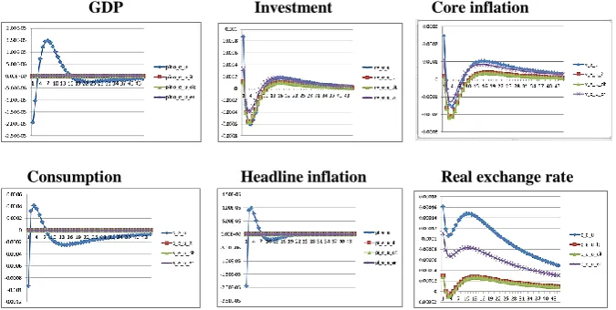
5. The Effect of External Shocks on Macroeconomic Variables

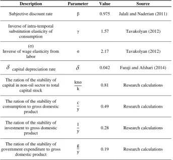
Given the major importance of external shocks for Iran's economy, the instantaneous response functions of the base model focus on them (Figure a 1, 2, and 3). In general, the cumulative macroeconomic responses are consistent with the structural characteristics of the Iranian economy. In addition, as our variables return after a relatively fast shock to a stable state, our model persists. Our analysis focuses on simultaneous responses to shock.

As expected, GDP, non-oil production will increase after a positive shock to oil prices. This response is consistent with the sensitivity of the economy to the oil sector. Negative response to oil production may depend on various factors. For this reason, the interpretation of the response is a difficult task. On the one hand, it may depend on the authorities' desire to limit oil supplies to maximize oil profits. On the other hand, as an OPEC member, Iran cannot freely adjust its oil supply in light of oil price changes. As a result, at least in the short term, oil production may be inextricably linked to price fluctuations. The shock of the oil price suggests a positive effect for consumers. Given the fact that officials are somewhat subsidizing domestic petroleum products, rising oil prices have little impact on consumer purchasing power. Sticky prices explain the immediate response to inflation due to the presence of subsidies and command prices. After the oil shock, the response is positive for both headline and core inflations. There is also a negative response to inflation in the import sector and the real exchange rate against the global oil price shock.

positive investment and non-oil production show a negative response to the depreciation of the euro against the dollar. Because the price of oil is expressed in dollars, the very high contribution of the oil sector to the GDP of Iran explains its positive response. The exchange rate shock is positive equivalent to a fortune. Increasing oil revenues, in turn, leads to an increase in non-oil production. Indeed, the non-oil sector is affected by the exchange rate shock through a policy of financial expenditures that is dependent on oil revenues. In other words, the volatility of the non-oil sector is significantly related to fluctuations in the oil sector. The exchange rate shock leads to a reduction in imported inflation, which in turn causes a negative response to headline and core inflation. As expected, consumption due to the shock of the exchange rate increases with respect to the positive effect of wealth. The real exchange rate is reduced due to the impact of the shock, but this is a short-term response. In the case of external shock, it should also be noted that this shock tends to exert a weak influence on domestic variables. This weak influence is based on the relatively low level of Iranian financial freedom.

Figure 1: Impulse Response Functions of Consumption, Investment and Exchange Rate against Simultaneous Shocks

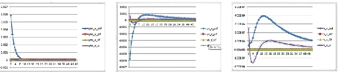
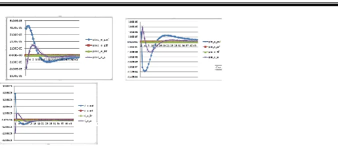
Figure 3: Impulse Response Functions of Headline Inflation, Core Inflation and Imported Inflation, against Simultaneous Shocks

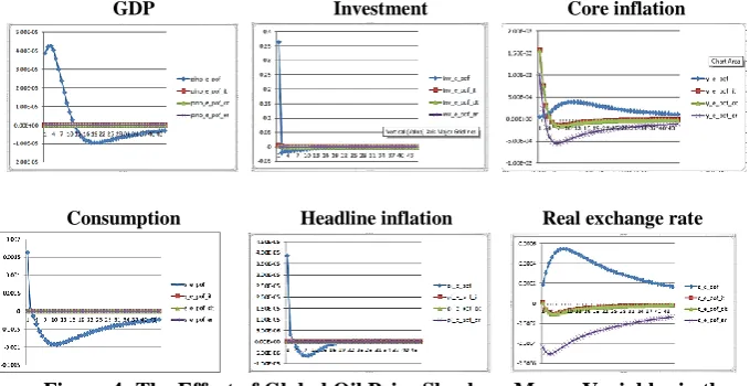
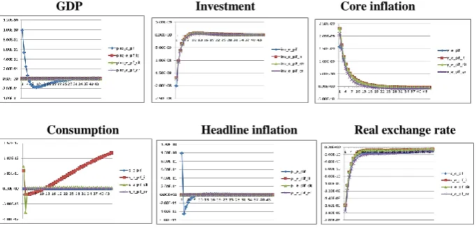
6. The Effect of External Shocks under Alternative Monetary Policy Rules

Forms B-1 to B-3 show our domestic macroeconomic responses to three shocks: oil prices, euro/dollar exchange rates and foreign inflation. We present the results for the base model and the three monetary policy principles, which include inflation targeting rule (IT rule), core inflation targeting rule (CIT rule), and exchange rate rule (ER rule). The importance of any monetary policy is deduced from the gap in the responses of our chosen variables in each form. When we consider the main shocks that are entering the country, the goal is to establish a monetary policy rule that minimizes both macroeconomic fluctuations and low inflation.

6.1 Effects of an Oil Shock

no significant difference for investment and GDP between the two inflation bases. However, we should take into consideration that immediate responses to the best policy rule for shocks influencing the economy are just one aspect of the matter, and the analysis of adjustments is also on the other side. Adjustment refers to the speed at which a particular variable returns to its sustainable level. Based on the base model and the exchange rate, real variables follow an unstable adjustment process. More precisely, our results show that short-run fluctuations are significant in these two scenarios, but the inflation-targeting rule and the core inflation-inflation-targeting rule did not significantly differentiate the process. Headline inflation and core inflation yield more combined results. In the case of shock effect, the maximum response to total inflation is obtained with the base model, while the core inflation-targeting rule and the initial response headline inflation are approximately equal to this shock, but the speed of modulation toward stability in core inflation is better. Therefore, our results indicate that the core inflation-targeting rule has little advantage over the inflation-targeting rule. Our results are in line with recent studies on monetary policy in small open economy (Paradou (2004); Madina and Soto (2005); and Dawen and Jesske (2007)).

GDP Investment Core inflation

Consumption Headline inflation Real exchange rate

Figure 4: The Effect of Global Oil Price Shock on Macro Variables in the form of Alternative Monetary Policy

6.2 Effects of EUR/USD Exchange Rate Shock

result in higher macroeconomic fluctuations than the other two. More precisely, real variables such as gross domestic product, consumption, investment, have more short-term response at the base of the exchange rate than core inflation targeting and headline inflation targeting. On the other hand, the two headline inflation and core inflation rules keep inflation at a very low level. In the comparison of core and headline inflation in response to the exchange rate shock, it should be said that the core inflation rate, in part, causes less fluctuations in macroeconomic variables compared to headline inflation. In addition, the results indicate that the central bank, if targeting the exchange rate rule, in response to this shock, faces many fluctuations in macroeconomic variables. However, the exchange rate rule is particularly effective in stabilizing the real exchange rate after a shock. However, when evaluating the agreeing and opposing reasons for alternative monetary rules, the effect should not be considered much for two major reasons: First, as shown in the figure, the real exchange rate response is short-term at any monetary rule. Second, as emphasized, the foreign exchange market of Iran is very small and the central bank is the only foreign exchange provider.

GDP Investment Core inflation

Consumption Headline inflation Real exchange rate

Figure 5: The Global Exchange Rate Shock on Macro Variables in the Form of Alternative Monetary Policy

6.3 Effects of Foreign Inflation Shock

on a relatively moderate level of Iran's financial freedom). In fact, in the case of an external shock, the response of many of the variables selected for the CIT rule to the two other monetary policy rules, namely, IT and ER rules, is negligible and ignored.

GDP Investment Core inflation

Consumption Headline inflation Real exchange rate

Figure 6: Impact of Global Inflation Shock on Macro Variables in the Form of Alternative Monetary Policy

7. Conclusions

shocks. It is suggested that Iran should adopt its monetary policy in order to adopt framework for core inflation targeting. This means that prerequisites such as the independence of the central bank must be realized. In this regard, Iran has been lagging behind other middle-income countries, especially the Middle East and North Africa, which prevents the use of interest rates as the main tool of monetary policy.

References

Allegret, J. P., & Benkhodja, M. T. (2015). External Shocks and

Monetary Policy in a Small Open Oil Economy. Journal of Policy

Modeling, 37, 652-667.

Bayat, N., & Bahrami, J. (2017). Evaluating Taylor Rule and Money

Growth Rate Rule in a DSGE Model for Iran. Iranian Journal of Trade

Studies, 8(21), 67-102.

Brock, W. A. (1974). Money and Growth: The Case of Long run Perfect

Foresight. International Economic Review, 15(3), 750-777.

Brock, W. A., & Lebaron, B. (1990). Liquidity Constraints in

Production-based Asset-pricing Models. In Asymmetric Information Corporate

Finance, and Investment. Chicago: University of Chicago Press.

Bouakez, H., Rebei, N., & Vencalachellum, D. (2008). Optimal Pass

Through of Oil Prices in an Economy with Nominal Rigidities. Working

Paper, 08/31, Retrieved from

https://papers.ssrn.com/sol3/Delivery.cfm/SSRN_ID1285503_code36 1712.pdf?abstractid=1285503&mirid=1.

Devereux, M., Lane, P. R., & Xu, J. (2006). Exchange Rate and

Monetary Policy in Emerging Market Economies. The Economic

Dhawan, R., & Jeske, R. (2007). Taylor Rules with Headline Inflation:

a Bad Idea. Federal Reserve Bank of Atlanta. Working Paper Series,

Retrieved from

https://papers.ssrn.com/sol3/Delivery.cfm/SSRN_ID998578_code362 125.pdf?abstractid=998578&mirid=1.

Dib, A. (2003). An Estimated Canadian DSGE Model with Nominal

and Real Rigidities. Canadian Journal of Economics, 36(4),949-972.

Faraji, M., Afshari, Z., & Ebrahimi, I. (2015). Oil Price Shocks and

Monetary Policy in Iran: the New Keynesian Approach. Journal of

Monetary and Banking Research, 22(7), 55-76.

Jalali Naeini, A. R., & Naderian, M. A. (2016). Monetary and Exchange

Rate Policy in An Oil Exporting Economy: The Case of Iran. Journal

of Monetary and Banking Research, 29(9), 1-21.

Ireland, P. (2004). A Method for Taking Models to the Data. Journal of

Economic Dynamics and Control, Retrieved from

https://www.sciencedirect.com/science/article/pii/S0165188903000800.

--- (2003). Endogenous Money or Sticky Prices? Journal of

Monetary Economics, 50, 1623-1648.

Kiyotaki, N., & Wright, R. (1993). A Search –theoretic Approach to

Monetary Economics. The American Economic Review, 83(1), 63-77.

Keynes, J. M. (1936). The General Theory of Employment, Interest and

Money. London: Macmillan.

Leduc, S., & Sill, K. (2004). A Quantitative Analysis of Oil Price

Shocks Systematic Monetary Policy and Economic Downturns. Journal

of Monetary Economics, 51,781-808.

Lucas, R. J. (1976). Econometric Policy Evaluation: A Critique.

Medina, J., & Soto, C. (2006). Copper Price, Fiscal Policy and Business

Cycle in Chile Central. Bank of Chile, Research Department, Retrieved

from

https://www.researchgate.net/profile/Claudio_Soto2/publication/2820 8383_Copper_Price_Fiscal_Policy_and_Business_Cycle_in_Chile/lin ks/02e7e52386d4f96651000000.pdf.

--- (2005). Oil Shocks and Monetary Policy in an Estimated

DSGE Model for a Small Open Economy. Central Bank of Chile,

Working Paper, 353, Retrieved from https://www.banqueducanada.ca/wp-content/uploads/2010/08/medina.pdf.

Mankiw, G., Romer, P., & Weil, D. (1992). A Contribution to the

Empirics of Economic Growth. Quarterly Journal of Economics,

2(107), 407-437.

Sidrauski, M. (1967). Rational Choice and Patterns of Growth in a

Monetary Economy. The American Economic Review, 57(2),534-544.

Tavakolian, H. (2013). A New Keynesian Phillips Curve in a DSGE

Model for Iran. Journal of Economic Research, 3(47), 1-22.

Tavakolian, H., & Sarem, M. (2017). DSGE Models in DYNARE.

Tehran, Monetary and Banking Research Institute, Retrieved from https://mbri.ac.ir/.

Tobin, J. (1977). How dead is Keynes? Economic Inquiry, 15, 459-468.

Walsh, C. (2003). Monetary Theory and Policy. Cambridge: MIT Press.

Yun, T. (1996). Nominal Price Rigidity, Money Supply Endogeneity,