in the population sciences published by the Max Planck Institute for Demographic Research Konrad-Zuse Str. 1, D-18057 Rostock·GERMANY www.demographic-research.org
DEMOGRAPHIC RESEARCH
VOLUME 18, ARTICLE 14, PAGES 409-436
PUBLISHED 27 MAY 2008
http://www.demographic-research.org/Volumes/Vol18/14/ DOI: 10.4054/DemRes.2008.18.14
Research Article
Constant global population with demographic
heterogeneity
Joel E. Cohen
c
°2008 Joel E. Cohen.
1 Introduction 410
2 The classical stationary population model 410
3 Heterogeneous stationary populations 412
3.1 Heterogeneous stationary populations: discrete case 412 3.2 Heterogeneous stationary populations: continuous case 416
3.3 Analytically soluble example 417
4 Constant global population with migration between countries 418 4.1 Alternative projections of a constant global population with
international migration 422
5 Demographic data 427
6 Acknowledgements 430
References 431
Appendix 1 433
Appendix 2 434
Constant global population with demographic heterogeneity
Joel E. Cohen1
Abstract
To understand better a possible future constant global population that is demographi-cally heterogeneous, this paper analyzes several models. Classical theory of station-ary populations generally fails to apply. However, if constant global population size
P(global)is the sum of all country population sizes, and if constant global annual num-ber of birthsB(global)is the sum of the annual number of births of all countries, and if constant global life expectancy at birth e(global) is the population-weighted mean of the life expectancy at birth of all countries, then B(global)·e(global) always ex-ceedsP(global)unless all countries have the same life expectancy at birth, in which case
B(global)·e(global) =P(global).
1Laboratory of Populations Rockefeller University & Columbia University 1230 York Avenue,
1. Introduction
In most countries of the world, human birth rates have been dropping and human life expectancies have been increasing (apart from countries severely afflicted by HIV-AIDS, economic disruption, and violent disorder). The end of global population growth lies within the range of plausible scenarios for the coming half-century or century (United Nations Population Division 2005). For example, in its low variant prepared in 2004, the UN Population Division projected that global population would peak in 2040 and then decline (until 2050, the horizon of the projection). In its medium variant, the pro-jected global net rate of reproduction fell to 1.00 by 2025-2030 and thereafter continued to decline, implying a future cessation of global population growth. Yet no demographic projections assume that all countries will have identical demographic characteristics.
It is therefore timely and useful to model a global population with unchanging total size and demographic variation among countries. This paper presents models of constant global populations and an apparently new inequality that connects population size, birth rates and life expectancy in a heterogeneous stationary population.
These models differ from graded models of stationary populations (e.g., Seal 1945; Vajda 1947; Bartholomew 1963; Keyfitz 1973), which assume that individuals advance through a linear succession of grades. Graded models have been used to study promotion in hierarchical organizations.
Coale (1972) emphasized that any earthbound population must have an average rate of growth that approaches zero as the time interval over which it is observed increases without limit, because infinite increase (implied by an average rate of increase that is pos-itive, no matter how small) is impossible on a finite Earth. Numerous models have been proposed to investigate how populations approach stationary size, including models with and without age structure, with and without migration among subpopulations, and with rates of birth, death and migration that are constant or changing in time (Espenshade 1978; Feeney 1971; Kim and Schoen 1996; Land and Rogers 1982; Le Bras 1971; Rogers 1968, 1990, 1995; Rogers and Castro 1981; Rogers and Henning 1999; Rogers et al. 2004; Ro-maniuc 2005; Schoen 1988, 2002; Schoen and Kim 1993, 1998-not an exhaustive list). These thoughtful and useful studies do not appear to have attained the results presented here.
2. The classical stationary population model
life table or survival function is the probability that a newborn individual survives to any given age or older, and is the complement of (i.e., one minus) the cumulative distribution function of length of life. The life tablel(x)depends on age only; it is assumed con-stant over time and applicable to all individuals. These attributes define a homogeneous stationary population.
A homogeneous stationary population arises in stable population theory from six con-ditions (Ryder 1975, p. 3): a fixed life table for females; a fixed maternity function for females; a net reproduction rate equal to 1; a fixed ratio of male to female births; a fixed survival function for males; and closure of the population to migration (this last condition can be relaxed). In the present paper, the assumptions about males will be ignored and a homogeneous stationary population will be treated as a single-sex model.
Three of the many well known properties of a homogeneous stationary population will be examined here.
First, in a homogeneous stationary population, if the life expectancyeis defined as the average number of years an individual lives from birth to death, thenP =Be(e.g., Keyfitz 1968, p. 7, Pollard 1973, p. 11). If the per capita crude birth rateb = B
P is the number of births per year per individual in the population, thenP =Beis equivalent to
1 = B
Pe=be or b= 1e.
Second, in a stationary population, leta∗be the age at which all individuals begin to
make a constant contribution ofcunits of money (e.g., dollars or Euros) per year to a re-tirement fund, letb∗be the age at which all individuals stop contributingcunits of money
per year to a retirement fund and start drawing a constant annuity of one unit of money per year from it, and letw∗be the maximum length of life in this population. Also letrbe the
interest or discount rate (assumed fixed and positive) so that one unit of money invested today is worth ertunits of money after tyears, or one unit of money to be received t years in the future has discounted present value e−rt. Then for a retirement system in balance (Alho and Spencer 2005, p. 84), the annual contribution every individual must make between agea∗andb∗to keep the retirement system in balance isc= A
D, where
A=
Z w∗
b∗
e−rxl(x)dx, D=
Z b∗
a∗
e−rxl(x)dx.
Herel(x)is the life table,Ais the expected present value at the birth of an individual of his or her retirement annuity, andcDis the expected present value at the birth of an individual of his or her lifetime contributions to the retirement system. Balance requires thatcD=A, hencec= AD.
Third, in a stationary population, let A be the average age, σ2 the variance of the
length of life (from birth to death), and (as before)ethe life expectancy (average length of life). ThenA= e+σ
2
e
3. Heterogeneous stationary populations
In a possible future, suppose each country has a homogeneous stationary population, but different countries have different life tables and birth rates, and migration between coun-tries is assumed to be negligible or zero. I define this situation to be a heterogeneous stationary population. In this model, the world has constant population size but the life expectancy of an individual depends on the country of birth.
A substantively different but formally equivalent heterogeneous stationary population is an honorific society with different classes of members (corresponding to different fields of learning or achievement) in which each class is permitted to elect a fixed number of new members per year, and members remain, until death, in the society and in the same class within the society. In the absence of changes in survival and in the absence of changes in the age distribution at election, each class will eventually become a stationary popula-tion. Different classes may elect different numbers of new members each year (each such election counts as a "birth" to the class) and may have different life expectancies (from election to death).
Given that the three identities above (P = Be,c = A D,A =
e+σ2
e
2 ) apply to each
country’s population (or each class’s membership) separately, do they also apply to the global population if each quantity on both sides of each equation is correctly aggregated from the corresponding quantities for each country? The answer established below is, somewhat unexpectedly, no. None of the three identities holds in general for the global population if each quantity on both sides of each equation is correctly aggregated from the corresponding quantities for each country. For the identitiesc= DA andA= e+σ
2
e
2 ,
inequalities may hold in either direction, depending on the example.
The main new positive finding below is that the first identity P = Beis a special case of an inequalityP ≤ Bein which equality holds if and only if all countries have identical life expectancies. In greater detail, suppose the population sizeP(global)is the sum ofP(country)for all countries, and the annual number of birthsB(global)is the sum ofB(country)for all countries, and the life expectancy at birthe(global)is the population-weighted mean ofe(country)for all countries. ThenB(global)·e(global)
always exceeds or overstatesP(global)unlesse(country)is the same for all countries.
3.1 Heterogeneous stationary populations: discrete case
country,xis the age in years,l(j,0) = 1andl(j, w∗) = 0), and life expectancy at birth
e(j) =
Z w∗
0
l(j, x)dx.
Then the stationary population size of countryjisP(j) =B(j)e(j), the global popula-tion size isPmj=1P(j)and the fraction of the global population in countryjisp(j)=PP(j). The global number of births per year isB =Pmj=1B(j). The global population’s life tablel(x)is the population-weighted mean of the country life tables
l(x) =
m
X
j=1
p(j)l(j, x);
Appendix 1 gives a detailed derivation. The global life expectancy is the population-weighted mean of the country life expectanciese=Pmj=1p(j)e(j).
We now prove that in a heterogeneous stationary population,Be≥P, andBe=P
holds if and only if all countries have the same life expectancy. Proof.
Be= [B(1) +. . .+B(m)][p(1)e(1) +. . .+p(m)e(m)]
= 1
P[B(1) +. . .+B(m)][P(1)e(1) +. . .+P(m)e(m)] = 1
P[B(1) +. . .+B(m)][B(1)e(1)
2+. . .+B(m)e(m)2]
≥ 1
P[B(1)e(1) +. . .+B(m)e(m)]
2
= 1
P[P(1) +. . .+P(m)]
2
=P.
The inequality follows from Cauchy’s inequality (Pólya and Szegö 1972, p. 68), stated in Appendix 2 below, withu(j) = pB(j)andv(j) = pB(j)e(j)forj = 1, . . . , m. Then equality holds if and only ife(j) is a constant independent ofj, i.e., if and only if all countries have the same life expectancy. QED
The life expectancy at birth of a randomly chosen person,e=Pmj=1p(j)e(j), differs in general from the life expectancy of a randomly chosen newborneb =
Pm
j=1b(j)e(j),
or countries’ shares of global births? The following hypothetical example suggests that countries’ shares of population are more appropriate weights. Suppose the world has
m = 2countries. Suppose each country is a stationary homogeneous population, and each has half the world’s births each year. In country 1, life expectancy at birth is 100 years, while in country 2, life expectancy at birth is 10 years. Consequently, country 1 has 10 times the population size of country 2. The life expectancy of a randomly chosen newborn is 100+10
2 = 55years, but the life expectancy of a randomly chosen person is 10
11 ·100 +111 ·10 = 91.8years as most of the world’s people are living in country 1. In
computing the global life expectancy, weighting each country’s life expectancy at birth by its share of population is intuitively as well as analytically the preferable alternative.
To examine the pension contributions and annuities in a heterogeneous stationary pop-ulation, we assume that all countriesj= 1, . . . , mhave the same first age of contribution
a∗, the same last age of contributionb∗, the same maximum length of lifew∗, and the
same discount rater. For countryj, the contribution per individual per year required to balance countryj’s retirement system isc(j) = DA((jj)), where
A(j) =
Z w∗
b∗
e−rxl(j, x)dx and D(j) =
Z b∗
a∗
e−rxl(j, x)dx.
Therefore the average annual contribution per person if each country balances its own retirement system is
c=
m
X
j=1
p(j)c(j) =
m
X
j=1
p(j) A(j) D(j).
The contributioncrequired per person using the global life table satisfiescD=Awhere
A=
Z w∗
b∗
e−rxl(x)dx= m
X
j=1
p(j)A(j)
and
D=
Z b∗
a∗
e−rxl(x)dx= m
X
j=1
p(j)D(j).
Hence
c=
m
P
j=1
p(j)A(j)
m
P
j=1
It is easy to generate numerical values ofp(j),A(j)andD(j)such thatc < cand other numerical values such thatc > c.
Similarly, let A(j)be the average age, σ2(j)be the variance of the length of life
from birth to death, and (as before)e(j)the life expectancy of countryj = 1, . . . , m. The variance of the length of life is the mean squared length of life minus the squared life expectancy. ThenA(j) = 1
2(e(j) +
σ2(j)
e(j) ). As before, the global life expectancy is
e=Pmj=1p(j)e(j)and the global average age is
A=
m
X
j=1
p(j)A(j)
=
m
P
j=1
p(j)e(j) + Pm
j=1
p(j)σe2((jj))
2
=
e+Pm
j=1
p(j) σe2((jj))
2 .
The global population’s variance of the length of life is the population-weighted mean of the countries’ mean squared length of life, minus the square of the population-weighted mean of the countries’ life expectancies, or
σ2=
m
X
j=1
p(j) (σ2(j) +e2(j))−(
m
X
j=1
p(j)e(j))2.
Thus we are interested in the relation between
A=
e+ Pm
j=1
p(j)σe2((jj))
2 and
e+σ2 e
2 ,
or equivalently (after cancelling the factor of 1
2 and removing the first termefound in
both expressions) in the relation between
m
X
j=1
p(j)σ
2(j)
e(j) and σ2
e .
As in the previous case, it is easy to generate numerical values ofp(j),σ2(j)ande(j)
such that Pm j=1
p(j)σe2((jj))< σ2
e and other numerical values such that m
P
j=1
While the three identities give useful information about a homogeneous stationary population, none of them necessarily holds for a heterogeneous stationary population. Two of the three identities may fail to hold in either direction, but the fundamental iden-tityP =Befor a homogeneous stationary population can be replaced by the inequality
P ≤Befor a heterogeneous stationary population, with equality if and only if all coun-tries have the same life expectancy.
3.2 Heterogeneous stationary populations: continuous case
A frequency histogram of the values of life expectancyewhere the unit of observation is a country summarizes international variation ine: the horizontal axis ise(discretized), and the height of the vertical bars represents the number of countries with life expectancy in the corresponding interval ofe. The total area under the frequency histogram (i.e., the sum of the heights of all the bars) ism, the number of countries. Now suppose the number
mof units of observation becomes large while the width of the bins used to calculate the frequency histogram becomes small in such a way that the shape of the frequency histogram, divided by its total aream, approaches a limiting probability density function
f(e)on the non-negative half line[0,∞). The probability density functionf(e)satisfies
R∞
0 f(e)de= 1. For example, instead of using a country as the unit of measurement, one
could measure the life expectancy of each province (primary administrative subunit) or of each county (secondary administrative subunit) worldwide. Asmincreases, it will be assumed that the number of units of observation with life expectancy in the interval from
e1toe2 > e1is increasingly well approximated bym Re2
e1 f(e)dewhile the total size of the heterogeneous stationary population remains constant atP. It will be assumed that the probability density functionf(e)and all other functions occurring here are properly integrable (as defined by Pólya and Szegö 1972, p. 46). For each life expectancye, the average number of annual births per country with life expectancyewill be represented by
B(e)≥0. It will be assumed further that the mean and variance ofB(e)with respect to
f(e)are finite. All of these assumptions are automatically satisfied in the discrete case and are reasonable assumptions for a continuous approximation to a demographically realistic situation.
Under the additional assumption that each unit of observation is a homogeneous stationary population, the population sizeP(e)of each unit with life expectancy eis
P(e) =B(e)e. Then the stationary global population size is the weighted sum over alle of the units’ population sizes,
P =m
Z ∞
0
The global number of births per year is
B=m
Z ∞
0
B(e)f(e)de.
As in the discrete case, the global life expectancy is the population-weighted mean of the life expectancies of each country. To avoid confusion with the dummy variableefor life expectancy, the symbolewill be used to denote the global life expectancy:
e= m
P
Z ∞
0
eP(e)f(e)de=m P
Z ∞
0
e2B(e)f(e)de.
By Schwarz’s inequality (Pólya and Szegö 1972, p. 68), which is the continuous version of Cauchy’s inequality,P ≤Be. In detail, Schwarz’s inequality states that ifu(x)and
v(x)are two functions that are properly integrable in the interval[a, b], then
(
Z b
a
u(x)v(x)dx)2≤
Z b
a
[u(x)]2dx
Z b
a
[v(x)]2dx.
Letu(e) =pB(e)f(e)andv(e) =epB(e)f(e). Then Schwarz’s inequality becomes
(
Z ∞
0
B(e)ef(e)de)2≤ Z ∞
0
B(e)f(e)de
Z ∞
0
e2B(e)f(e)de
or(P
m)2≤ Bm·P em which simplifies toP ≤B e. QED
As in the discrete case, the inequality does not depend on the numbermof countries or other units of observation.
3.3 Analytically soluble example
To confirm and quantify the inequalityP ≤ B ein an analytically soluble, hypothet-ical example of the continuous case of a heterogeneous stationary population, suppose that the probability density function (pdf) of the country life expectancyeis the gamma distribution with parametersρ(a positive real number) andr(a positive integer),
f(y) = ρ
re−ρyyr−1
(r−1)! ,
for ally≥0. Initially assumer >1. The caser= 1will be considered separately. IfY
is a random variable with gamma pdff(y), then forn= 0,1,2, . . .,
E(Yn) =
Z ∞
0
ynf(y)dy=(r+n−1)
(n)
where(a)(n)=a(a−1)· · ·(a−n+1)is the falling factorial, e.g.,(a)(0)= 1,(a)(1) =a,
(a)(2)=a(a−1). SupposeB(e) = 1
e (hereerepresents life expectancy, not the base of natural logarithms) so that the births per year in each country are (in some arbitrary units) inversely proportional to the life expectancy of that country. ThenB(e)e= 1soP =m
ande= m
P E(Y) = rρ. Also
B =m
Z ∞
0
1
yf(y)dy
=m
Z ∞
0
ρre−ρyyr−2
(r−1)! dy
=m ρ r−1
Z ∞
0
ρr−1e−ρyyr−2
(r−2)! dy =m ρ
r−1
since the last integrand on the right is the gamma pdf with parametersρandr−1. There-foreB e=m r
r−1 > m. The inequality is expected from the general inequalityP ≤B e.
Whenr = 1, the gamma distribution becomes the exponential distribution so that
P=mande= m
PE(Y) = 1ρ, but
B =m
Z ∞
0
1
yf(y)dy=m
Z ∞
0
ρ e−ρyy−1dy
which diverges to infinity, so the inequalityP < B e holds.
At the other extreme, ifr→ ∞, thene→ ∞andB →0whileB e↓mso that the inequality approaches equality. In the gamma pdf with parametersρandr, the coefficient of variation, i.e., the standard deviation divided by the mean, isr−1
2, which approaches 0 as r → ∞. Thus the demographic interpretation of the case when r → ∞ is that global life expectancy grows longer on average and, relative to this increasing average, also grows less variable from country to country.
4. Constant global population with migration between countries
In a heterogeneous stationary population, each country has constant size and no individu-als migrate from one country to another, by assumption. We now consider a discrete-time model of a constant global population with migration among countries. In this model, countries may change size in time. Later we will give a hypothetical numerical example.
sizes) att. For the country of originiand the country of destinationj, wherei 6=j, let
M(i, j, t)≥0be the number of migrants from countryito countryjbetweentandt+ 1, defined as the number of people who were in countryiattand in countryj (different fromi) att+ 1. (Thisde factodefinition does not coincide with the legal definition of a migrant used by many countries.) LetM(i, i, t) = 0for alli. Them×mmatrixM(t)
with elementsM(i, j, t)is called the migration matrix.
The number of emigrantsE(i, t)from countryibetweentandt+ 1is the number of people who were in countryiattand were elsewhere att+ 1, namely, the sum of rowiof the migration matrix:E(i, t) =PjM(i, j, t)≥0. The number of immigrantsI(i, t)to countryibetweentandt+ 1is the number of people who were elsewhere than country
iattand were in countryiatt+ 1, namely, the sum of columniof the migration matrix:
I(i, t) =PhM(h, i, t)≥0.
The number of net migrants to countryibetweentandt+ 1is
N(i, t) =I(i, t)−E(i, t) =X
h
M(h, i, t)−X
j
M(i, j, t). (1)
Net migration is positive if immigration exceeds emigration, zero if immigration equals emigration and negative if emigration exceeds immigration. ThenN(t), the sum of net migrants over all countries, is guaranteed to be zero (with no further assumptions) because
N(t) =X
i
N(i, t) =X
i
I(i, t)−X
i
E(i, t) =X
h,i
M(h, i, t)−X
i,j
M(i, j, t) = 0.
Each country’s population may change as a result of migration and vital events (i.e., births and deaths): fori= 1, . . . , m,
P(i, t+ 1) =P(i, t) +N(i, t) +B(i, t)−D(i, t), (2)
whereB(i, t)is the number of births andD(i, t)is the number of deaths betweentand
t+ 1in countryi. To assure thatP(i, t+ 1)≥0, it will be required that
P(i, t)≥D(i, t)−B(i, t)−N(i, t).
If each term in equation (2) is summed over all countriesi= 1, . . . , m, and ifB(t)is the sum of births andD(t)is the sum of deaths in all countries betweentandt+ 1, then becauseN(t) = 0, we have
P(t+ 1) =P(t) +B(t)−D(t).
The assumption thatB(t) = D(t) is a significant constraint, as the following hy-pothetical scenario illustrates. If all migrants were people past the ages of childbearing and if they all moved from a high-mortality country to a low-mortality country and im-mediately acquired that lower rate of mortality, as will be further assumed below, then
D(t+1)< D(t)and global births would also have to decrease, even though the migration involved only people past childbearing. This problem arises only if the model has age structure.
If each country were modeled as having its own age structure and its own life table, then it would be necessary to specify the age structure of migrants (e.g., Rogers 1968, 1995; Rogers and Castro 1981; Rogers and Henning 1999; Rogers, Castro and Lea 2004). To avoid tracking ages, we now make the further simplifying assumption that, for each countryj, for each interval fromttot+ 1, and for every agex, countryjhas a force of mortalityµ(j, t)(also called the per capita instantaneous death rate or hazard of mortality) that applies to every individual while that individual lives in countryjduring the interval fromt tot+ 1. The force of mortality applies equally to natives and to immigrants, assuming that, upon migration, migrants change instantaneously and completely from the life table of the country of origin to the life table of the country of destination. The period life expectancye(j, t)of countryjis then 1
µ(j,t)during the time interval fromttot+ 1.
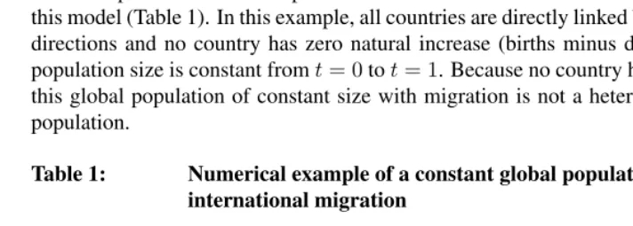
A simple numerical example illustrates some of the main features and limitations of this model (Table 1). In this example, all countries are directly linked by migration in both directions and no country has zero natural increase (births minus deaths), yet the total population size is constant fromt= 0tot= 1. Because no country has unchanging size, this global population of constant size with migration is not a heterogeneous stationary population.
Table 1: Numerical example of a constant global population with international migration
time t=0 t=1
country i P(i,0) M(i,1,0) M(i,2,0) M(i,3,0) E(i,0) N(i,0) B(i,0) D(i,0) P(i,1) country 1 20 0 2 3 5 5 1 2 24 country 2 30 4 0 5 9 0 6 3 33 country 3 50 6 7 0 13 -5 5 7 43 total 100 10 9 8 27 0 12 12 100
=I(1,0) =I(2,0) =I(3,0)
Table 2: Numerical example of births, life expectancy and population size in a stationary population with migration
time t=0 t=1 t=1/2 t=1/2 t=1/2 t=1/2 country i P(i,0) P(i,1) P(i,1/2) D(i,0) e(i,0) B(i,0) b(i,1/2) d(i,1/2)
country 1 20 24 22 2 22
2= 11 1 221 222
country 2 30 33 31.5 3 31.5
3 = 10.5 6 316.5 313.5
country 3 50 43 46.5 7 46.5
7 = 6.64... 5 465.5 467.5
total 100 100 100 12 100
12= 8.33... 12 10012 10012
Symbols are defined in Table 1 note.
Table 2 continues the numerical example from Table 1. Becausee(j, t) = 1
µ(j,t) and
µ(j, t) = person-years lived , the life expectancyD(j,t) e(j, t)of countryjis the person-years lived betweentandt+ 1divided by the numberD(j, t)of deaths betweentandt+ 1. The person-years lived are determined by the exact timing of events of migration, birth and death betweentandt+ 1. A reasonable linear approximation to person-years lived is the average of the population in the country attand att+ 1,P(j,t)+P2(j,t+1), denoted
P(j, t+ 1
2)for brevity. Hencee(j, t) =
P(j,t+1 2)
D(j,t) is the (approximate) life expectancy
of countryjbetweentandt+ 1. Then the life expectancye(t)of the global population betweentandt+ 1is the weighted average of the life expectancy in each country. The weights are person-years lived in each country divided by the sum of the person-years lived over all countries. The period life expectancye(t)>0betweentandt+ 1reflects births, deaths and migration because all three factors affect the person-years lived between
tandt+ 1. In this example, the global life expectancy is
22·11 + 31.5·10.5 + 46.5·46.5 7
100 =
222
2 +31.5
2
3 +46.5
2
7
100 = 8.816
> P(t) B(t) =
100
12 = 8.333,
which is the estimate of the global life expectancy that would be obtained assuming a
homogeneousstationary population and ignoring differences among countries.
In general, in a constant global population with migration between countries, for each year[t, t+ 1]considered separately, B(t)e(t) ≥ P(t+ 1
B(t)e(t) = P(t)holds if and only if all countries have the same life expectancy. The proof (in Appendix 2) parallels the proof in a heterogeneous stationary population, except that here the Cauchy-Schwarz inequality is applied to the person-years lived instead of to the population attort+ 1. These results depend on the assumption thatB(t) =D(t)at each time.
A similar inequality holds when averaging over time as well as over countries. The time-average birth rate and the time-average life expectancy of the global population from 0 toT are
B = 1
T
TX−1
0
B(t), e= 1 T
TX−1
0
e(t).
ThenP ≤B e, andP < B eunless all countries have equal life expectancies at all times. These results depend on the assumption thatB(t) =D(t)at each time. The proof is in Appendix 3.
4.1 Alternative projections of a constant global population with international migration
Suppose we have complete data for each country in the world on each country’s popula-tion size at timestandt+ 1and its immigrants and emigrants and births and deaths from
ttot+ 1, and suppose global population sizeP(t) = P(t+ 1)is constant. How shall we project future population sizes globally and by country? For a recent review of some projection techniques in use, see Howe and Jackson (2005).
The remainder of this subsection offers three linear ways of projecting the future of a constant global population with international migration and shows by numerical example that all three approaches have problems. The three approaches assume that
(i) the change in the population of each country is constant over time, or
(ii) demographic rates relative to the population of the sending country are constant (a sender-controlled linear representation), or
(iii) demographic rates relative to the population of the receiving country are constant (a receiver-controlled linear representation).
All three methods can give exactly the same population sizes of all countries att= 0and
t = 1. The three methods may give very different projections of the future fromt = 2
that further work is needed to develop a useful projection method for a constant global population with international migration.
We now present the analysis and numerical example in detail. Equations (1) and (2) and the remainder of this section are independent of any assumption that the life table is exponential or otherwise. We may rewrite the definition of net migration in equation (1) as
N(i, t) =X
h
M(h, i, t)−E(i, t) =X
h6=i
P(h, t)M(h, i, t)
P(h, t) −P(i, t) E(i, t) P(i, t).
Letb(i, t) = BP((i,ti,t)) be the crude birth rate per capita and letd(i, t) = DP((i,ti,t))be the crude death rate per capita of countryi fromttot+ 1. (The denominators are intentionally
P(i, t)and notP(i, t+1
2).) Then
P(i, t+ 1) =P(i, t) [1−E(i, t)
P(i, t)+b(i, t)−d(i, t)] +
X
h6=i
P(h, t)M(h, i, t) P(h, t) .
Define, for i = 1, . . . , m,a(i, i, t) = 1− EP((i,ti,t)) +b(i, t)−d(i, t), and forh 6= i,
h= 1, . . . , m,a(h, i, t) = MP((h,i,th,t)). The off-diagonal elements of the matrix a are thus nonnegative. (In the numerical example, the matrixais computed in Table 3.) Then equation (2) is equivalent to
P(i, t+ 1) =
m
X
h=1
P(h, t)a(h, i, t), i= 1, . . . , m (3)
which is a donor-controlled linear representation of a constant global population with international migration. Then the global population size is the same attandt+ 1:
m
X
i=1
P(i, t+ 1) =
m
X
h=1
P(h, t)
m
X
i=1
a(h, i, t)
=
m
X
h=1
P(h, t) [a(h, h, t) +X
i6=h
a(h, i, t)]
=
m
X
h=1
[P(h, t)−E(h, t) +B(h, t)−D(h, t) +X
i6=h
M(h, i, t)]
=
m
X
h=1
=
m
X
h=1
[P(h, t) +B(h, t)−D(h, t)]
=
m
X
h=1
P(h, t).
Dividing both sides by the global populationP and lettingp(i, t) =P(Pi,t) gives
p(i, t+ 1) =
m
X
h=1
p(h, t)a(h, i, t), i= 1, . . . , m.
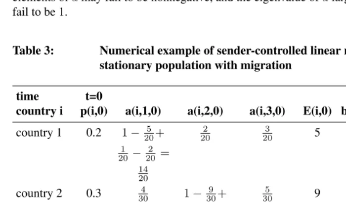
Unlike a time-inhomogeneousm-state Markov chain (e.g., Iosifescu 1980), here neither the row sums nor the column sums of the transition matrixaare required to be 1, and the elements ofamay fail to be nonnegative, and the eigenvalue ofalargest in modulus may fail to be 1.
Table 3: Numerical example of sender-controlled linear representation of a stationary population with migration
time t=0 t=1
country i p(i,0) a(i,1,0) a(i,2,0) a(i,3,0) E(i,0) b(i,0) d(i,0) p(i,1)
country 1 0.2 1− 5
20+ 202 203 5 201 202 0.24 1
20−202 = 14 20
country 2 0.3 4
30 1−309+ 305 9 306 303 0.33 6
30−303 = 24 30
country 3 0.5 6
50 507 1−1350+ 13 505 507 0.43 5
50−507 = 35 50
total 1.0 0.9533... 1.04 1.0166... 27 12 12 1
Whenever the matrixais nonnegative and some power of it has strictly positive el-ements (as in the numerical example in Table 3), the Perron-Frobenius theorem (e.g., Gantmacher 1960) assures that the proportion of global population found in each coun-try will converge to a constant fraction and that the size of the global population and of each country will eventually change by a constant factor each year. That factor of annual change is given by the eigenvalue of theamatrix with maximal absolute value (the so-called spectral radius of theamatrix), which is guaranteed to be a positive real number. The long-run proportions of global population in each country are given by the elements of the eigenvector corresponding to the spectral radius normalized to sum to 1. Although the matrix ais constructed to assure that global population remains constant between
t = 0andt = 1, there is no guarantee that when the matrixais assumed constant the global population size will remain constant beyondt= 1in the short term or long term. Unless the spectral radius of the matrixahappens to be 1, the global population and each country’s population will not be stationary in the long run.
In the numerical example in Table 3, the three eigenvalues ofa are approximately 1.0086, 0.6298 and 0.5616, hence the spectral radius of theamatrix is 1.0086. Con-sequently after projecting each country’s population a long time assuming a constanta
matrix, the population of each country and of the world will increase by about 0.86% per year. From the last two lines of Table 5, in the projection assuming a constantamatrix, the annual increase of country 1’s population is100·(3130..1283 −1) = 0.93% (using the original projection before rounding), of country 2’s population 0.90%, and of country 3’s population 0.75%. The rates of increase for all three countries fromt = 99tot = 100
are all 0.86%, as expected from the spectral radius ofa.
Rewriting (2) in the form (3) represents the number of migrants as proportional to the size of the population of the sending country. An obvious alternative is to represent the number of migrants as proportional to the size of the population of the receiving country. Rewrite (1) as
N(i, t) =I(i, t)−X
j
M(i, j, t) =P(i, t)I(i, t) P(i, t)−
X
j6=i
P(j, t)M(i, j, t) P(j, t)
so that
P(i, t+ 1) =P(i, t) [1 + I(i, t)
P(i, t)+b(i, t)−d(i, t)]−
X
j6=i
P(j, t)M(i, j, t) P(j, t) .
Define, fori= 1, . . . , m, z(i, i, t) = 1 + PI((i,ti,t))+b(i, t)−d(i, t), and forj6=i,
j = 1, . . . , m, z(i, j, t) =−MP((i,j,tj,t)), so that all off-diagonal elements of the matrixz
Then (2) is equivalent to
P(i, t+ 1) =
m
X
j=1
z(i, j, t)P(j, t), i= 1, . . . , m, (4)
which is a receiver-controlled linear representation of a constant global population with international migration. Dividing both sides by the total populationP and letting
p(i, t) = P(Pi,t)gives
p(i, t+ 1) =
m
X
j=1
z(i, j, t)p(j, t), i= 1, . . . , m.
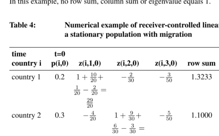
In this example, no row sum, column sum or eigenvalue equals 1.
Table 4: Numerical example of receiver-controlled linear representation of a stationary population with migration
time t=0 t=1
country i p(i,0) z(i,1,0) z(i,2,0) z(i,3,0) row sum b(i,0) d(i,0) p(i,1) country 1 0.2 1 + 10
20+ −302 −503 1.3233 201 202 0.24 1
20−202 = 29 20
country 2 0.3 −4
20 1 + 309+ −505 1.1000 306 303 0.33 6
30−303 = 42 30
country 3 0.5 −6
20 −307 1 + 508+ 0.5867 505 507 0.43 5
50−507 = 56 50
total 1.0 10 9 8 3.0100 12 12 1 =I(1,0) =I(2,0) =I(3,0)
Note:p(i, t)= fraction of global population in countryiatt,z(i, j, t)=receiver-controlled migration matrix att (see text for definition)
in the population of countryiis constant for allt, equation (2) gives a projection tech-nique. If one assumes the matrix ais constant for all t, equation (3) gives a sender-controlled projection technique. If one assumes the matrixzis constant for allt, equation (4) gives a receiver-controlled projection technique. When the matrices are related as above, all three methods give exactly the same population sizes of all countries att= 0
andt = 1. In this numerical example, the three methods give very different projections of the futuret= 2, . . .(Table 5).
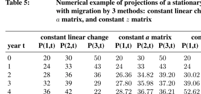
Table 5: Numerical example of projections of a stationary population with migration by 3 methods: constant linear change, constant
amatrix, and constantzmatrix
constant linear change constantamatrix constantzmatrix year t P(1,t) P(2,t) P(3,t) P(1,t) P(2,t) P(3,t) P(1,t) P(2,t) P(3,t) 0 20 30 50 20 30 50 20 30 50
1 24 33 43 24 33 43 24 33 43
2 28 36 36 26.36 34.82 39.20 30.02 37.10 33.26
3 32 39 29 27.80 35.98 37.20 39.06 42.61 19.59
4 36 42 22 28.72 36.77 36.21 52.62 49.88 0.28
5 40 45 15 29.35 37.36 35.78 72.96 59.28 −27.11
6 44 48 8 29.82 37.83 35.68 103.46 71.12 −66.09
7 48 51 1 30.20 38.24 35.75 149.25 85.48 −121.65
8 52 54 −6 30.53 38.62 35.93 218.01 101.99 −200.97
9 56 57 −13 30.83 38.98 36.17 321.37 119.28 −314.29
10 60 60 −20 31.12 39.33 36.44 476.89 134.15 −476.24
Note:P(i, t)= population of countryiat start of yeart. Matricesaandzare defined in text.
5. Demographic data
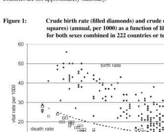
birth rate exceeds the death rate, so (ignoring international migration) the population is growing and has a younger age structure than it would if it were stationary with the same life table. The crude death rate falls below the reciprocal of the life expectancy. Most countries are not approximately stationary.
Figure 1: Crude birth rate (filled diamonds) and crude death rate (open squares) (annual, per 1000) as a function of life expectancy (years) for both sexes combined in 222 countries or territories
Note:Apparently filled squares represent the coincidence of a crude birth rate and crude death rate. Countries with missing data are excluded. Dashed line shows 1000/life expectancy, the theoretical prediction for both birth rate and death rate (per 1000) in a homogeneous stationary population.
Source of data:Reference Bureau DataFinder, http://www.prb.org/datafind/datafinder7.htm, accessed 2006-08-11
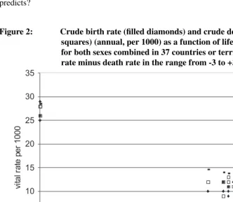
in magnitude, specifically, in the range from -3 to +3 per thousand. Does the reciprocal of the life expectancy predict well the crude birth rate and the crude death rate in coun-tries where these rates are nearly equal, as the homogeneous stationary population model predicts?
Figure 2: Crude birth rate (filled diamonds) and crude death rate (open squares) (annual, per 1000) as a function of life expectancy (years) for both sexes combined in 37 countries or territories with birth rate minus death rate in the range from -3 to +3 per thousand
Note:Apparently filled squares represent the coincidence of a crude birth rate and crude death rate. Countries with missing data are excluded. Dashed line shows 1000/life expectancy, the theoretical prediction for both birth rate and death rate (per 1000) in a homogeneous stationary population.
Source of data:Reference Bureau DataFinder, http://www.prb.org/datafind/datafinder7.htm, accessed 2006-08-11
av-erage estimated for the world as a whole, where crude birth rates and crude death rates fall below the reciprocal of life expectancy. Ryder (1975, p. 4) called the first group countries with "inefficient" replacement and the second group countries with "efficient" replacement. It remains to be seen whether countries with efficient replacement will be better described by the stationary population model in the future.
6. Acknowledgements
References
Alho, J. and Spencer, B. (2005).Statistical Demography and Forecasting. Springer, New York.
Bartholomew, D. (1963). A multi-stage renewal process.J. R. Statist. Soc., B 25:150–168. Coale, A. (1972). Alternative paths to a stationary population. In Westoff, C. and Parke, R., editors,Demographic and Social Aspects of Population Growth. U.S. Commission
on Population Growth and the American Future, research reports vol. 1., pages 589–
603. Government Printing Office, Washington, DC.
Espenshade, T. (1978). Zero population growth and the economies of developed nations.
Popul. Devel. Rev., 4:645–680.
Feeney, G. (1971). Comment on a proposition of H. Le Bras. Theor. Popul. Biol., 2:122– 123.
Gantmacher, F. (1960). Theory of Matrices.Chelsea, New York.
Howe, N. and Jackson, R. (2005). Projecting immigration: a survey of the current state of practice and theory. A Report of the CSIS Global Aging Initiative, with contributions by Rebecca Strauss and Keisuke Nakashima. Center for Strategic and International Stud-ies, Washington, DC. http://ideas.repec.org/p/crr/crrwps/2004-32.html, last accessed 2008-02-20.
Iosifescu, M. (1980).Finite Markov Processes and Their Applications. John Wiley, New York, Editura Tehnica, Bucharest.
Keyfitz, N. (1968). Introduction to the Mathematics of Population. Addison-Wesley, Reading.
Keyfitz, N. (1973). Individual mobility in a stationary population. Popul. Stud., 27:335– 352.
Kim, Y. and Schoen, R. (1996). Populations with sinusoidal birth trajectories. Theor.
Popul. Biol., 50:105–123.
Land, K. and Rogers, A., editors (1982). Multidimensional Mathematical Demography.
Academic, New York. pages 477-503.
Le Bras, H. (1971). Équilibre et croissance de populations soumises à des migrations.
Theor. Popul. Biol., 2:100–121.
Marshall, A. and Olkin, I. (1979). Inequalities: Theory of Majorization and its
Applica-tions.Academic Press, New York.
Pollard, J. (1973). Mathematical Models for the Growth of Human Populations. Cam-bridge University Press, CamCam-bridge.
Pólya, G. and Szegö, G. (1972). Problems and Theorems in Analysis, Vol. I: Series,
Inte-gral Calculus, Theory of Functions.Springer-Verlag, New York, Heidelberg, Berlin.
Preston, S., Heuveline, P., and Guillot, M. (2001). Demography: Measuring and
Rogers, A. (1968). Matrix analysis of interregional population growth and distribution.
University of California Press, Berkeley.
Rogers, A. (1990). Requiem for the net migrant.Geogr. Anal., 22:283–300.
Rogers, A. (1995).Multiregional demography: principles, methods and extensions.John Wiley, New York.
Rogers, A. and Castro, L. (1981). Model migration schedules. Research Report-81-30. International Institute for Applied Systems Analysis, Laxenburg.
Rogers, A., Castro, L., and Lea, M. (2004). Model migration schedules: three alterna-tive linear parameter estimation methods. Institute of Behavioral Science, Research Program on Population Processes, University of Colorado at Boulder, Working Paper POP2004-0004.
Rogers, A. and Henning, S. (1999). The internal migration patterns of the foreign-born and native-born populations in the United States: 1975-80 and 1985-90.Int. Migr. Rev., 33:403–429.
Romaniuc, A. (2005). Stationary population as theoretical concept and as policy vision for Canada. Presented at workshop on "Population Changes and Public Policy", London, Ontario, Canada, February 3-4, 2005. sociology.uwo.ca/popchange/Romaniuc,%20 Stationary%20population.pdf.
Ryder, N. (1975). Notes on stationary populations.Popul. Index, 41:3–28. Schoen, R. (1988).Modeling Multigroup Populations. Plenum Press, New York. Schoen, R. (2002). On the impact of spatial momentum. Demographic Res., 6:49–66.
www.demographic-research.org/Volumes/Vol6/3/.
Schoen, R. and Kim, Y. (1993). Two-state spatial dynamics in the absence of age.Theor.
Popul. Biol., 44:67–79.
Schoen, R. and Kim, Y. (1998). Momentum under a gradual approach to zero growth.
Popul. Stud., 52:295–299.
Seal, H. (1945). The mathematics of a population composed of k stationary strata each recruited from the stratum below and supported at the lowest level by a uniform annual number of entrants.Biometrika, 33:226–230.
United Nations Population Division (2005). World Population Prospects: The 2004 Re-vision, Highlights, ESA/P/WP.193, 24 February 2005. Department of Economic and Social Affairs. United Nations, New York.
Appendix 1
The global population’s life table is the population-weighted mean of the country life tables, i.e.,l(x) =Pmj=1p(j)l(j, x).
Proof.
LetX be a continuous, real nonnegative-valued random variable that represents an individual’s length of life or exact age at death. Then the global probability of surviving from birth to agexor longer isl(x) =P[X≥x]. The conditional probability of surviv-ing from birth to agexor longer, given residence in countryj, isl(j, x) =P[X≥x|j]. Everybody in the global population lives in some country (by assumption). Each coun-try’s life table applies to all individuals in that country regardless of theircurrent age, by definition. The decomposition formula for conditional probabilities isP[X ≥x] =
Pm
j=1P[X≥x|j]p(j). This is the same asl(x) = Pm
Appendix 2
Cauchy’s inequality: Letu(1), . . . , u(m),v(1), . . . , v(m)be arbitrary real numbers. Then
[u(1)v(1) +. . .+u(m)v(m)]2≤[u(1)2+. . .+u(m)2] [v(1)2+. . .+v(m)2].
Equality holds if and only if for some real constantsλandµwithλ2+µ2>0we have
λ u(j) +µ v(j) = 0 forj= 1, . . . , m.
Jensen’s inequality (e.g. Marshall and Olkin 1979, p. 454): For any real interval(a, b)
and any convex functionf defined on(a, b)and any real numbersu(1), . . . , u(m)each in(a, b)and any nonnegative real numbersv(1), . . . , v(m)such thatPmj=1v(j) = 1, one has
f(Xu(j)v(j))≤Xv(j)f(u(j)).
Jensen established an integral analog using Lebesgue measure.
In a constant global population of sizeP(t)with migration between countries, ifB(t) =
D(t)for all t, then for each year[t, t+ 1]considered separately,
B(t)e(t)≥P(t+1
2) =P(t) =P(t+ 1),
andB(t)e(t) =P(t)holds if and only if all countries have the same life expectancy.
Proof.
The indices i, j run over all countries from 1 to m. Write t0 = t+ 1 2 so that
P(j, t0) = P(j,t)+P(j,t+1)
2 is the person-years lived in countryj fromt tot+ 1. Then
the global life expectancy is
e(t) =
P
jPP(j, t0)e(j, t)
iP(i, t0)
=
P
j P(j,t0)2
D(j,t)
P(t0)
=
P
j( P(j,t0)
√
D(j,t)) 2
Hence
B(t)e(t) =D(t)
P
j( P(j,t0)
√
D(j,t)) 2
P(t)
=X
i
D(i, t)
P
j( P(j,t0)
√
D(j,t)) 2
P(t)
=X
i
p
D(i, t)2
P
j( P(j,t0)
√
D(j,t)) 2
P(t)
≥
(PjpD(j, t)√P(j,t0)
D(j,t)) 2
P(t)
=P(t)
2
P(t) =P(t)
Appendix 3
In a constant global population of sizeP(t)with migration between countries, ifB(t) =
D(t)for allt, then the time-average birth rateB = 1
T
PT−1
0 B(t)and the time-average
life expectancye= 1
T
PT−1
0 e(t)of the global population from 0 toT satisfyP ≤B e,
andP < B eunless all countries have equal life expectancies at all times.
Proof.
By the result in Appendix 2, the fixed global population sizeP =P(0)>0satisfies, for everyt= 0,1, . . . , T, B(t)e(t)≥P, with equality if and only if all countries have the same life expectancy betweentandt+ 1.
Henceforth the lower and upper limits of summation are 0 andT −1, respectively. SinceB(t)≥ P
e(t)for everyt= 0,1, . . . , T−1,
B= 1
T
X
B(t)≥ P T
X 1
e(t)≥ P
1
T
P
e(t)= P
e.
The first inequality above follows from Cauchy-Schwarz and is strict if and only if, for at least onet, at least two countries have different life expectancies. The second inequality follows from Jensen’s inequality (Appendix 2) and is strict unlesse(t)is constant fort
from 0 toT−1.
In detail, on the positive real line, 1
y is a strictly convex function ofy. By Jensen’s inequality, the average of the reciprocal ofyis greater than or equal to the reciprocal of the average ofy, and the inequality is strict if and only ify takes at least two distinct values each with positive measure. In particular, takingy(t) =e(t)gives
X 1
e(t)≥ 1
P
e(t)