Predicting order lead times

Paper received: 13.9.2007 Paper accepted: 19.12.2007

Predicting Order Lead Times

Tomaž Berlec* - Edvard Govekar - Janez Grum - Primož Potočnik - Marko Starbek University o f Ljubljana, Faculty o f Mechanical Engineering, Slovenia

Entering on market, companies confront with different problems. But the largest problems o f today's time are too long lead times o f orders. A client that wants a particular product to be made will select the best bidder considering on delivery time.

To make a bid ju st on the basis o f experience o f employees is very risky nowadays. Therefore we propose a procedure by which - on the basis o f actual lead times o f orders processed in the company's workplaces in the past - expected lead times o f planned (and indirectly - production) orders can be predicted. The result o f the proposed procedure is an empirical distribution ofpossible lead times fo r the new order, and on the basis o f this distribution it is possible to predict the most probable lead time o f a new order. Using the proposed procedure, the sales department can make a prediction fo r the customer about delivery time o f the planned order.

As an illustration o f the procedure fo r predicting lead times o f orders, a case study is presented: lead time o f orderfor the "toolfor manufacturing the filter housing" was predicted; the tool is manufactured in the Slovenian company ETI Ltd.

© 2008 Journal o f M echanical Engineering. All rights reserved.

Keywords: lead times, prediction, operation order, empirical distribution

0 INTRODUCTION

C om panies on the g lo b al m arket offer similar or the same products at comparable price and quality. The main difference between these companies is in the predicted order development time and in observance o f the deadlines for delivery time.

Before making a bid, the sales department has to provide data on operations that will have to be carried out for a particular order, data on the time required for performing these operations, and data on requested delivery time. Currently, the data at times o f realization o f operations are obtained from experienced company employees, while the c u sto m e r sp e c ifie s d e liv e ry tim e. H ow ever, estim ates based on personal experience can be rather misleading. Consequently, the bids may be based on wrong delivery time which can couse that the company does not receive the order.

Development o f ICT - which are important reso u rces fo r im p ro v in g and m aintaining the com petitive advantages o f the com pany on the market [ 1 ] - made radical changes as ICT simplifies many business-related tasks. Every company that wants to be competitive on the global market needs a suitable enterprise resource planning system - ERP system . T h ere are several ERP system s

available on the market [2] and it is the task o f each company to select the optimum system [3].

The paper will present how the data stored in the ERP system can be used for calculation o f lead times o f orders (and indirectly: lead times o f m anu factu rin g orders) on the basis o f theory d ev elo p ed at the IFA H an n o v er [4] and [5], F urtherm ore, the calculation o f percentage o f m anufacturing order lead tim es will be shown, w hich allows the calculation o f the confidence interval. The purpose o f this paper is therefore to propose a procedure for predicting lead times o f manufacturing orders on the basis o f past gathered data on actual lead times.

In o u r research w e have n o t fo u n d an approach for predicting lead times as described in this paper, so we assume that it is a new approach which uses already known and developed theory o f IFA H annover, and adds a new m ethod for predicting order lead times.

1 METHOD FOR PREDICTING MANUFACTURING ORDER LEAD TIMES

W hen ta lk in g a b o u t “ an o rd e r” , it is n ecessary to distinguish betw een operational, manufacturing, assembly and production order [4], as presented in Figure 1.

SD,

SK,

SD2

I

s d3

Manufacturing order lead time

Manufacturing order lead time

'

Assembly order lead time

.

Production order lead time

---Jr

Fig. 1. Order lead times [4]

When designing a procedure for predicting manufacturing order lead times, it will be assumed that the com pany uses an ERP system , w hose database contains data about past operational and assembly orders in company workplaces. Any ERP system should therefore provide data on:

• production-order code, • assembly-order code, • manufacturing-order code, • operational-order code,

• ty p e and seq u e n c e o f o p e ra tio n s on manufacturing and assembly orders,

• IDs o f workplaces where operational orders have been carried out,

• actual execution times of operational orders, • date o f completing a particular operational or

assembly order in the previous workplace, • date o f finishing a particular operational or

assembly order in the observed workplace. ERP system output data should be available in Microsoft Excel format (xls).

Based on previous research on problems of determination o f lead times let us to the conclusion,

that the proposed procedure for predicting order lead times consists of the following steps:

Step 1: Determining actual lead times of already processed operational orders in the company’s workplaces

H. P. Wiendahl [4] says that the lead time o f the /-th operational order N. (1 < i < n) which has been executed in the /-th workplace DM. (1 < j< m) is defined as an interval, calculated from the time when the /-th operational order has been completed in the previous, i.e. (j-l)-th workplace, till the time when the /-th operational order has been completed in the observed, i.e.y-th workplace (Fig. 2). Lead time of an operational order is therefore:

TOi,j = t K I J - t K UH) (1),

TO - lead time of the /-th operational order in the

7

tK - completion time o f the /-th operational order in the /-th workplace

tK . I) - completion time o f the /-th operational order in the previous (J-l)-th workplace

O - i )

TPREg Jf/ Z F J tK'J Time [Wd or Cd]

TO,, !

Fig. 3. Flow o f operational orders through the DM. workplace [4]

i - operational order number

j - workplace number

On the basis o f the ERP system output data it is possible to calculate (for any y-th workplace

DMj) the actual lead times o f previously executed o p eratio n al orders, i.e. orders th a t have been processed in they'-th workplace in the observed time interval P (Fig. 3).

The actual lead times o f operational orders, executed in the y-th workplace in the observed time interval are therefore:

TOy j = tKy j tKy^j—J)

TOi.j = tK2j -tKi.u-i)

TOn,j - tKn.j

n - number o f processed operational orders in the past on i-th workplace

m - number o f workplaces

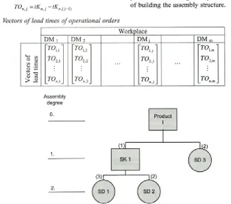
Vectors of actual lead times o f operational o rd ers, ex ecu ted in the p a st in all com p an y w orkplaces (table 1), will present the basis for predicting expected lead times o f the planned new production orders.

Step 2: Forming assembly structure of the planned production order and technology routings for parts and components of planed order

The assem bly structure and technology routings o f realization o f com ponent parts and assemblies o f manufacturing orders are made on the basis o f available documentation o f the planned production order. Figure 4 presents the principle o f building the assembly structure.

Table 1. Vectors o f lead times o f operational orders

Work place

DM i DM 2 DM, DM m

V

e

c

to

rs

o

f

le

a

d

t

im

e

s

TOu

TOu

TOnX

TOy 2

TO 1 :2

T ° n , 2 .

TOy.:

TO,,

T ° n , _

TOlm '

T 0 lml , m

TOnm

Assembly degree

Legend: I - product

SK - mark o f asembly SD - mark o f component part

(x) - number o f built ins o f component parts and assemblies in assembly o f higher degree

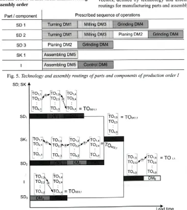
Figure 5, presents technology and assembly routings for manufacturing parts and components o f the production order I.

Step 3: Random sampling and summing of vector element values of actual lead times of operational orders of individual manufacturing or assembly order

Figure 6 presents the principle of random sampling and summing o f vector element values o f operational order actual lead times in the past of planned manufacturing and assembly orders. TOSD1, - lead time o f component part SD]( got after

first iteration

TOsk, , - lead time o f assembly SK,, got after first iteration

TO ,, - lead time o f product I, got after first iteration Figure 6 shows a schematic presentation o f random sampling and addition o f lead times values achieved in the past from w orkplace vectors, defined by technology and assem bly routings for manufacturing parts and assembly o f

Part / component Prescribed sequence of operations SD 1 Turning DM1

ill

_{IliH l l i l M}

SD 2 Turning DM1 Milling DM3 P,a„mgD M 2

I ailbfii*

SD 3 Planing DM2 | Gn

fl||

_■

SK 1 Assembling DM5

I Assembling DM5 Control DM6

Fig. 5. Technology and assembly routings o f parts and components o f production order I

S D ; S K

S K ,

S D ,

[t o,,;

F

T O , ,3 T Oi,4 T O , , , t o2i3

\

T 0 2 ,4

[ T O n . y T O n ,3

\

S D 3

T O

1.5

| T O

n,5

: T Osk

T O ,.! T O,,3 t o, ; t o, ;

T O ,,, _{T 0 2,3} t o2,2 T 0 2,4 _{T O s 0,},

TO„,, "

.

I

■

0

] «HI

c

•

O

H

I

0

■

p

Ito , ! to , i4

to2 i 2 % to 2 .4

[to J \ tOm =

T O , T 0 2 ,

T ° n ,(

: T O sD3,1

T O j T 0 2 ,6

5 J ° n , j I dm 6

: TO 1.1

Lead time

SD; SK A

VsD

1

TOsm,i TOsD1,2

TOsDt.k

--- ► Lead time

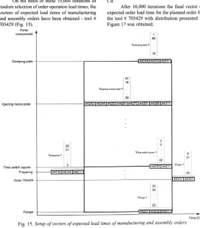
Fig. 7. Setting up vectors o f expected lead times ofplanned manufacturing and assembly orders

com ponents.

It is necessary to select the num ber o f iterations fo r ra n d o m s a m p lin g o f le a d tim e s o f m anufacturing and assem bly orders o f planned p ro d u c tio n o rd e r (co m p u ter su p p o rted ). The num ber o f iterations is affected by the order type — by increasing its com plexity, the num ber o f iterations should be increased, too.

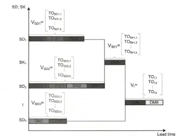
Step 4: Setting up vectors of expected lead times o f m a n u f a c t u r in g and a sse m b ly orders of planned order

Results o f step 3 allow setup o f vectors of the expected lead times o f the manufacturing and assembly orders o f planned production order, as presented in Figure 7.

TOSD1 k - lead time o f component part SD p got after k - th iteration

V SDl — lead time vector o f assembly SDj k - num ber o f iteration

The number o f elements in individual vector depends on the number o f performed iterations k. The number o f required iterations can be established on the basis o f tests, as it is necessary to assure a stable process, which cannot be achieved by a small number o f iterations. A criterion for an adequate number o f iterations is that multiple use o f the procedure must

yield comparable results, by which the stability (convergence) o f the procedure is achieved.

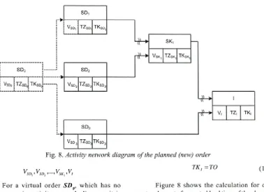
Step 5: Definition of vector of expected lead times of the planned order

In order to define the vector of expected lead tim es o f the planned production order V t, it is necessary to transform the Gantt chart of production order (Fig. 7) into an activity network diagram o f order and enter into it the vectors o f expected lead tim es o f manufacturing and assembly orders o f planned order (Fig. 8).

Initial data o f activity network diagram o f planned order are:

• date o f starting the execution o f the virtual order

SDq

-TZSDo= 0 (4),

v e c to r o f the v irtu a l m a n u fa c tu rin g and assembly order VSD0 is:

V,S D 0 (5),

S D o

j Vso» T Zsdj T Ksd,

S D ,

VsDi —1 N _5? T Ksd,

s d2

Vsd2 T Zsd2 T Ks d2

s d3

v s d3 T Zsd3 T KsDj

#-►

S K ,

VsK 1 T Zsk, w"

X

H

4 " - > i

n f - V| T Z , TK,

Fig. 8. Activity network diagram o f the planned (new) order

V V V V

,s d i >vs d2 ’ ■■ ■’ v S K , ’ v 1

F or a v irtu al order SD 0, w hich has no predecessors in activity network diagram , it is assumed that the date o f starting the execution o f order is (for the first iteration):

TZSDo<= 0 (6),

and the date o f finishing the execution o f order is

TKm =TZ,n +TO,n_{■ "•'} = 0 + 0 = 0 (V).

0.1 ■ "•'0.1 ■ "•'0.1

For o th e r m a n u fa c tu rin g o r assem b ly orders, which have one or more predecessors (Fig. 9) is the date o f starting the execution o f orders then:

, = max jrZ JD + TOsd j (8)

o .i k e p a. I

P* - predecessors o f the observed order N

and the date o f finishing the execution o f orders

TKsDb, = TZsDb, + TOSDt, (9).

Date o f completing the last manufacturing or assembly order I is equivalent to the expected lead time of the planned order TO in the activity network diagram:

TK,=TO (io).

Figure 8 shows the calculation for one vector element o f expected lead time o f the planned order. Such a calculation must be done for a selected number o f iterations o f randomly sampled values from vectors o f individual component partsand assemblies o f planned order. The calculation is carried out as follows:

• For sequential operations, individual randomly sampled lead times from vectors o f sequentially listed workplaces are summed up. The result o f each iteration is stored into a new vector, which represents the sum for one component or part.

• For parallel operations it is necessary to collect randomly sampled lead times from vectors of parallel workplaces, and then find a maximum lead time for each parallel path. Thus obtained results in each iteration should be stored in the common vector o f maximum times o f parallel paths, as the critical path in the activity network diagram is always the path with the longest req u ired lead tim e for re a liz a tio n the manufacturing order.

SDa SD„

r *

---w

S

V)

>

TZsob.1 TKsDb.1

C a lc u la tio n has to be re p eated for the selected number o f iterations.

Thus obtained expected lead times o f the planned order will represent empirical distribution o f lead times o f the planned order.

Step 6: Predicting delivery time of the planned order

Step 5 in predicting order lead time has lead to the vector o f expected lead times o f order, i.e. to a certain distribution o f lead times.

In real life, however, an exact value o f lead time for delivery o f order is required.

The m ost probable delivery lead time for the p lan n ed o rd er can be estim ated by u sing m e d ia n , w h ic h m ean s th a t th e re is a 50% probability that the actual delivery time will be shorter, and 50% probability that it will be longer than stated. As the 50% risk is usually unacceptable for the client, so the estim ated value should be stated for a w ider confidence interval.

For instance, 90% confidence interval is defined as 90% probability that the order will be d e liv e re d b e fo re the sta te d tim e. T h erefo re, maximum delivery time that can be guaranteed to the customer with 90% reliability, corresponds to the 90th percentage o f empirical distribution o f prediction o f the planned order.

Percentage [6] and [7] provides the value o f ¥, which is larger than P % o f the values in the X

set. In other words, e.g. 90th percentage gives the value, which is larger than 90% o f all values (sorted from smallest to largest) in the X set (Fig. 10).

In order to obtain the P -th percentage o f X

sorted values, it is necessary to calculate the R rank

[8]:

R = P(X+1)/100 (11),

which is rounded to the first integer and then the value from the X set is selected, which corresponds to this rank.

R - percentage rank P - percentage

X - number o f sorted set elements

Based on the above explanation and our tests, we propose that the 90th percentage be used as a standard. In this way it is possible to state with 90% confidence that the order will be completed within the expected time.

I f the company wants to achieve even higher reliability, it can use an even higher percentile (for example 99th) - and thus minimize the risk.

Naturally, the choice o f the percentage may depend on importance o f the order and the customer - the more important the customer, or the more important the order, the higher is the interest o f the company to get a particular order.

In the proposed procedure for predicting manufacturing order lead times, in addition to MS Excel, the MATLAB software will be used [6], which allows execution o f mathematical operations and graphical presentation o f results.

2 TESTING THE PROCEDURE FOR PREDICTING ORDER LEAD TIMES

The procedure for predicting order lead tim es w as tested in the to o l shop o f ETI Ltd. company from Izlake, Slovenia. It produces tools for transform ing and cutting, tools for injection m o u ld in g o f th e rm o p la s tic and d u ro p la stic materials, je t and press machines for duroplastic

Lead time of

materials, press machines for ceramic materials, and automated assembly appliances.

This tool shop speciality is design and manufacturing o f high-quality tools for injection m o u ld in g o f th e rm o p la stic and d u ro p la stic materials. Thanks to its many years of experience in making tools for ETI company, the tool shop started producing tools and appliances for external custom ers in the follow ing fields: autom otive in d u stry , h o u se h o ld a p p lia n c e s, m e d ical technology, electrical engineering, electronics and illumination.

Tool shop u ses L argo ERP sy stem , developed by Perftech Ltd. company from Bled [9], Slovenia. Because o f their way o f production (tools are made for known customers and each tool is unique) it is very difficult to precisely predict duration o f production - but this is essential data for making bids and winning orders.

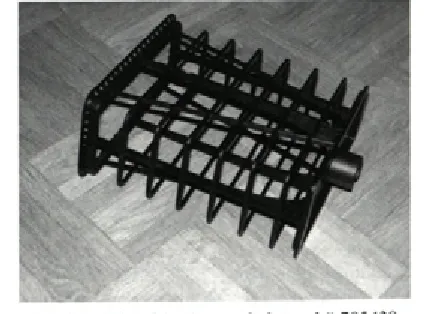
Company management decided to test the suitability o f the proposed procedure for predicting lead times o f orders in a case study o f determining lead time o f order for the “tool for manufacturing filter housing # 705429” (Fig. 11).

Steps o f the p ro ced u re fo r p re d ic tin g manufacturing order lead time for the “tool for manufacturing filter housing # 705429”:

Step 1: D eterm ining actual lead tim es of operational orders finished in the past in the company’s workplaces

For the experiment, the Largo ERP system data were used in the period from December 12, 2002 till August 22, 2005.

First it was necessary to export data from Largo ERP system to MS Excel form at. The

following data were exported from the database: o rd er num ber, a rriv a l date, d e p a rtu re date, manufacturing time, and sequence o f operational orders.

Largo ERP system uses calendar dates and does not take into account the company’s labour- days calendar. Therefore the data which are not adapted to the company’s labour days are useful mainly for predicting the duration of production from the sales department’s point o f view and not that much for manufacturing planning - for this purpose it would be necessary to take into account the company’s labour-days.

In a g reem en t w ith the tool shop management it was decided that for determining actual lead times o f operational orders finished in the past, the data from the ERP system would be used from December 12,2002 till August 22,2005. During that time, 22,850 manufacturing orders were processed in the production, with 57,951 operational orders in 35 workplaces (Table 2).

It can be seen that during the observed time a rather varying num ber o f operational orders passed across workplaces (minimum o f 2 orders over w orkplace 44321 and m aximum o f 7307 orders over workplace 44253).

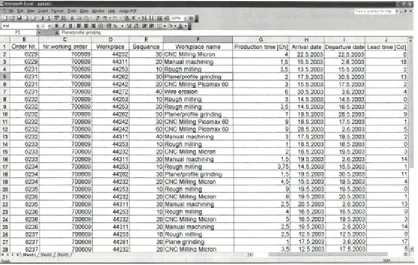
Actual lead times o f individual operational orders were calculated on the basis o f the data obtained from the ERP system. The calculation was made in MS Excel on the basis o f Equation (1). Figure 12 presents a part o f the calculation o f actual lead times o f operational orders in Excel table.

The results have shown that majority o f actual lead tim es shorter then 1 Cd or 1 Cd, exceptions to the rule are some extreme cases, e.g. 464 Cd.

Table 2. Number o f operational orders finished on workplaces in the tool shop

Code: W orkplace name:

N um ber o f finished orders in three years:

44000 Cooperation - service 21

44141 Design o f devices 151

44142 M achine electronics 130

44143 Design o f tools 2288

44211 Slitting 1420

44221 Turning 3706

44222 CNC turning 1052

44231 CNC programming 371

44232 CNC M illing M icron 2660

44241 CNC programming 668

44242 CNC M illing Picomax 60 4153

44243 CNC programming 9

44244 CNC M illing Deckel Maho 1400

44251 CNC M illing Picomax 54 2018

44252 M illing 235

44253 Rough milling 7307

44261 Plane grinding 1972

44262 Plane/profile grinding 4225

44263 Round grinding 2894

44264 Tools sharpening 159

44265 CNC coordinate grinding 7

44271 CNC programming o f wire erosion 1126

44272 W ire erosion 1927

44273 W ire erosion -M akino 3161

44281 Dip erosion - AGIE 439

44282 Dip erosion - Charmilles 1565

44283 Dip erosion - Sinitron 513

44286 Omega punching 745

44291 Heat treatment 5172

44311 M anual machining 4288

44312 Assem bly o f tools 812

44313 A ssem bly o f machines and devices 197

44321 Sampling 2

44331 M easurement 885

44332 DEA Omicron measurem ent 273

Three years production: 57951

Step 2: Using or forming assembly structure of the planned order and technology routings of parts and components of order - for tool # 705429

In this step known assem bly structure is form ed (Fig. 13), as w ell as know n type and sequence o f operations (Fig. 14) for the tool under discussion - tool # 705429.

It can be seen from Figure 13 that the tool consists o f two parts: ejecting and feeding part. The tool consists o f bought parts and of parts/components made in the tool shop. There is just one assembly operation at the end, which is followed by testing.

| g Microsoft Excel - podatki

: -1} 0 e 6 * ifiew insert Format loots Data V£ndcm (jefc Adobe PDF Type a q i« te n k e nep » . » x

1 4 ^ :V f S

i* a ( s • » . / ■ * » * :<ä ■* • . a i a : * *

1 Arial _{i - 8 7 « » .# * a i9 ..v .jc a *.*}

_____ ! Plane/profile grinding

B C D E F G H 1 J

1 Order Nr. Nr.working order Workplace Sequence W orkplace name Production time [Eh] Arrival date Departure date Lead time [Cd]

2 6229 700609 44232 30 CNC Millinq Micron 4 22.5.2003 22.5.2003 0

3 6229 700609 44311 201Manual machininq 1,5 15.5.2003 2.6.2003 18

4 6231 700609 44253 10 Rouqh millinq 3,5 13.5.2003 15.5.2003 2

5 6231 700609 44262 30 Plane/profile qrindinq 2 17.5.2003 30.5.2003 13

6 6231 700609 44242 20 CNC Millinq Picomax 60 3 15.5.2003 17.5.2003 2

7 6231 700609 44272 40 Wire erosion 6 30.5.2003 3.6.2003 4

8 6232 700609 44253 10 Rouqh millinq 3 14.5.2003 14.5.2003 0

9 6232 700609 44253 20 Rough millinq 3,5 14.5.2003 16.5.2003 2

10 6232 700609 44262 50 Plane/profile qrindinq 7 19.5.2003 28.5.2003 9

11 6232 7006091 44242 30 CNC Milling Picomax 60 9 16.5.2003 17.5.2003 1

12 6232 700609! 44242 60 CNC Millinq Picomax 60 9 28.5.2003 2.6.2003 5

13 6232 700609 44311 40 Manual machininq 3 17.5.2003 19.5.2003 2

14 6233 700609 44253 ___ 10] Rough millinq 1 16.5.2003 16.5.2003 0

15 6233 700609 44232 20 CNC Millinq Micron 2 16.5.2003 19.5.2003 3

16 6233 700609 44311 30 Manual machininq 1,5 19.5.2003 2.6.2003 14

17 6234 700609 44253 10 Rough millinq 3,75 14.5.2003 15.5.2003 1

18 6234 700609 44262 30 Plane/profile grindinq 1,5 19.5.2003 30.5.2003 11

19 6234 700609 44232 20 CNC Millinq Micron 4,5 15.5.2003 19.5.2003 4

20 6235 700609 44253 10 Rouqh millinq 9 19.5.2003 19.5.2003 0

21 6235 700609 44232 20 CNC Millinq Micron 6 19.5.2003 20.5.2003 1

22 6235 700609 44311 30 Manual machining 2,5 20.5.2003 2.6.2003 13

23 6236 700609 44253 10 Rouqh millinq 4 16.5.2003 16.5.2003 0

24 6236 700609 44232 20 CNC Millinq Micron 5 16.5.2003 19.5.2003 3

25 6236 700609 44311 30 Manual machininq 2,5 19.5.2003 2.6.2003 14!

26 6237 700609 44253 10 Rouqh millinq 2,5 12.5.2003 12.5.2003 0

27 6237 700609 44261 30 Plane qrindinq 1 17.5.2003 3.6.2003 17

28 6237 700609 44232 20 CNC Millinq Micron 3.5 12.5.2003 17.5.2003 5

M i► M\Sheet 1 / Sheet2 / Sheet3 / |< »

Fig. 12. Calculation o f actual lead times offinished operational orders in interval from December 12, 2002 till August 22, 2005

provide quality parts and components. For the tool # 705429 some o f these data are presented in Figure 14.

In tool shop in ETI L td. they do an conglomeration o f operations named preparing on m anufacturing, w hich for this order contains: m achine electro n ics (44142), design o f tools (44143) and slitting (44211). This is actually not a real part o f the tool, which can be shown in Figure 14, but it consumes time, so it is necessary to count it in by the sequence o f operations.

Steps 3 and 4: Random sampling and summing of vector element values of actual operational order lead times of individual manufacturing or assembly order of the planned order, and setup of vectors of expected lead times of manufacturing and assembly orders of the planned order for the tool # 705429

On the basis o f defined sequence of machining on parts and components for the tool # 705429 made by MATLAB software, the vectors o f expected lead

Parts/components Sequence of operations

Preparing 4 4 1 4 2 4 4 1 4 3

... I ^ ::U...\Ì 44211 J

Clamping plate 44244 4 4 3 1 1

Ejecting modul ₄₄₂₄₄ 4 4 3 1 1

Final switch square 4 4 3 1 1

Flange 4 4 2 2 1 4 4 2 3 2 4 4 3 1 1

Order 705429 4 4 3 1 2 4 4 3 1 1

B

e

rl

e

c

T

.

-

G

o

v

e

k

a

r E.

-

Gr

um

J.

- P

o

to

č

n

ik

P

.

-

S

ta

rb

e

k

M

.

Assembling H p j level:

Note: All component parts made in this tool shop, have the first treatment named preparing, which for this order contains: Machine electronics (44142), Design o f tools (44143) and Slitting (44211).

S

tr

o

jn

iš

k

i v

e

st

n

ik

-

Jo

u

rn

a

l

o

f M

e

c

h

a

n

ic

a

l

E

n

g

in

e

e

ri

n

g

5

4

(2

0

0

8

)5

,

3

0

8

-3

2

times o f manufacturing and assembly orders have been set up, as described in the theoretical part of this paper. On the basis o f tests with 500, 1000, 5000, 10,000,20,000 and 50,000 iterations we concluded th a t the p re d ic tio n p ro cess s ta b iliz e s at approximately 10,000 iterations. If much fewer iterations are used, predictions are unstable, as insufficient data are used. If many more than 10,000 iterations are selected, the data used are repeated, so the result is not any better, while the processing time increases. We therefore used 10,000 iterations during a random selection of lead times.

On the basis o f these 10,000 iterations o f random selection o f order operation lead times, the vectors of expected lead times o f manufacturing and assembly orders have been obtained - tool # 705429 (Fig. 15).

Step 5: Definition of vector of expected lead times of the planned manufacturing order for the tool # 705429

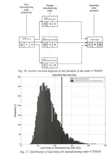
10,000 ite ra tio n s w ere m ade fo r the calculation o f expected lead tim e vector o f the planned order for the tool # 705429. A sam ple calcu latio n o f lead tim e for one iteratio n is presented in Figure 16. Expected lead tim e o f the planned order is calculated as the sum o f tim e o f preparing, m axim um tim e o f parallel m a n u fa c tu rin g o rd e rs, and assem b ly o rd er, w hich in our case am ounts to 16 + 28 + 9 = 53 Cd.

After 10,000 iterations the final vector o f expected order lead time for the planned order for the tool # 705429 with distribution presented in Figure 17 was obtained.

Parts/ com ponents

C lam ping plate

Ejecting m odul plate

Final switch square P reparing

O rde r 705429

Flange

I 25 51

Vpreparing = |

I 3 i

Vclamping plate =

16 !

14 4 1 4 2 1 4 4 1 4 3 144211

-4 44244144253TTOTT

41

I 16 ;

V e jectin g module plate —

34 .

4424214424414425314426t 144272144251144256144311

V fin a l switch square

-22

—I 44253 1443T T V o rd e r

-5 I

21

Vfla ng e -33 34

22

-144221144432144TTT

J_20

44312 1 44331~1

Fig. 16. Activity network diagram o f one iteration o f the order # 705429

estimated total lead time

3 5 0 i---1--- 1--- --- i

Lead times of manufacturing order [Cd] «■■■ 90% confidence interval

■ j distribution of lead tim e fo r m anufa ctu ring order

Fig. 17. Distribution o f lead times fo r manufacturing order # 705429

Step 6: Predicting delivery time of the planned tool production order # 705429

In the fifth step the vector o f lead time of the planned order (i.e. distribution o f lead times of order) was set. However, no customer is interested in a lead-time vector (or distribution o f lead times), so as the first approximate delivery time value, the

median o f this vector is used; for this order it is:

TO _{m ed}= 77 Cd

TOmed - median lead time o f the tool production order # 705429

Confidence intervals are defined according to the selected confidence levels.

If a very high confidence level is required, the 90th percentage is used. So, for the order # 705429 it can be stated with 90% confidence level that this order will be produced within

TO** =120 Cd

Togo«/,, - lead time at 90th percentage

The company has to decide itself, which risk level it is ready to accept when signing the contract with the customer.

3 CONCLUSION

D ue to ev e r fie rc e r c o m p e titio n o f companies on domestic and foreign markets, and due to transition from the market o f sellers to the m arket o f custom ers, the com panies have to continuously reduce delivery times o f the order.

The p a p e r p ro p o se s a p ro c e d u re for predicting manufacturing order lead times on the basis of past actual lead times of operational orders. The use o f the proposed procedure allows: • prediction o f lead time needed for delivery o f

any new order,

• variation o f delivery-time calculations on the basis o f acceptable risk level by selecting the confidence interval.

The basis for calculation o f delivery time is median, while 90th percentage may represent the upper (safe) lim it, w hich can be offered to the customer as the latest delivery lead time. On the basis o f its experience and its willingness to risk, the com pany can choose different confidence interval.

The procedure for predicting order lead times has been tested in a case study o f predicting lead times for producing a tool for manufacturing a filter casing in the tool shop o f the ETI Ltd. Case study was performed on the basis o f data, defined in calendar days collected in three years in the data base o f ERP system Largo.

By using th is p ro ced u re o f pred ictin g manufacturing order lead times, sales department can make a well-defined bid for the customer in a

short time without the sales person needing many years of experience - (s)he only needs well-defined tech n o lo g y ro u tin g s, w hile the com p an y management provides the confidence interval.

In the future it is planned that the proposed procedure will be improved by taking into account the sequence o f operations required to complete an order, the influence o f the number o f operations per order, the influence o f manufacturing time, etc.

Acknow ledgem ents

We would like to thank to the tool shop of ETI Ltd. company for disposal o f the data from their ERP system, for their help. We would also like to thank to the Slovenian Ministry of Higher Education, Science and Technology for their financial aid during development o f this method.

4 REFERENCES

[1] Leem, C.S., Suh, J.W. Techniques in integrated development and implementation o f enterprise information systems. Intelligent Knowledge-Based Systems, Business and Technology in the New Millennium, voi. 2, 2005, p. 3-26. [2] Scherer, E. ERP - Projekte auf dem Prüfstand

der Praxis. ERP M anagement, GITO mbH Verlag, 2005, p. 34-37.

[3] S tarbek, M ., G rum , J. S e lectio n and implementation o f a PPC system. Production Planning & Control, 2000, vol. 11, p.765-774. [4] Wiendahl H.P. Load-oriented manufacturing control. Berlin: Springer Verlag, 1995, p. 37-199. [5 ] N yhuis, P., W iendahl, H.P. L o g istisch e

Kennlinien. Berlin: Springer Verlag, 1999, p. 81-94.

[6] Getting Started with MATLAB. The Math Works, Inc., ver. 6, 2002.

[7] Rice, A.J. M athematical statistics and data analysis, 2nd Ed. California: International Thomson Publishing, 1995.

[8] h ttp ://en.w ikipedia.org/w iki/P ercentile, 25 November 2006.