Regression Analysis of Dissolved Heavy Metals in Storm Water Runoff from Elevated Roadways

(1)

University of New Orleans Theses and

Dissertations Dissertations and Theses

5-21-2005

Regression Analysis of Dissolved Heavy Metals in Storm Water

Runoff from Elevated Roadways

Ruben Erlacher

University of New Orleans

Follow this and additional works at: https://scholarworks.uno.edu/td

Recommended Citation Recommended Citation

Erlacher, Ruben, "Regression Analysis of Dissolved Heavy Metals in Storm Water Runoff from Elevated Roadways" (2005). University of New Orleans Theses and Dissertations. 150.

https://scholarworks.uno.edu/td/150

This Dissertation is protected by copyright and/or related rights. It has been brought to you by ScholarWorks@UNO with permission from the rights-holder(s). You are free to use this Dissertation in any way that is permitted by the copyright and related rights legislation that applies to your use. For other uses you need to obtain permission from the rights-holder(s) directly, unless additional rights are indicated by a Creative Commons license in the record and/ or on the work itself.

(2)

A Dissertation

Submitted to the Graduate Faculty of the University of New Orleans in partial fulfillment of the requirements for the degree of

Doctor of Philosophy in

The Engineering and Applied Science Program

by

Ruben Erlacher

D.I., University of Innsbruck, 2002 M.S., University of New Orleans, 2001

(3)

ii

ACKNOWLEDGEMENTS

I would like to express my sincere gratitude to my advisor, Dr. Marty

Tittlebaum from the Department of Civil and Environmental Engineering, who’s advice,

support, and friendship have provided me with an invaluable source of motivation over

the last three years. His way of teaching with great sense of humor and his incredible

knowledge and experience in his field has encouraged me very much and will be

exemplary for my whole life.

Moreover, I am grateful to Dr. Donald E. Barbé, Dr. Bhaskar Kura, Dr. Paul

Gremillion and Dr. Ronald Stoessel, for serving on my Ph.D Examining Committee and

providing me with further assistance.

I would also like to thank my friends Armin Gschnitzer and Oscar Vera Moronta,

without whose help my research work would not have been successful.

Important, I would especially like to thank my parents, whose love and great

support was indispensable, and who have provided me with lifetime motivation and

inspiration.

My greatest appreciation goes to my girlfriend Carmen Walder, whose boundless

love, kindness and sensitivity I will never forget and to whom I would like to dedicate

(4)

iii

LIST OF FIGURES

Figure 1. pH Values of Common liquids ...67

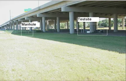
Figure 2. View of the Experimental Site and Manhole...80

Figure 3. Plan View of the Specific Drainage Area (6,288 ft²) of the Selected Highway Section of Interstate-610 in Orleans Parish, New Orleans, Louisiana ...81

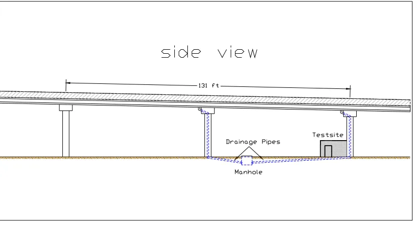
Figure 4. Side View of Section through the Selected I-610 Highway Section at the Experimental Site ...81

Figure 5. The Experimental Site beneath the East-Bound Lane of the I-610...82

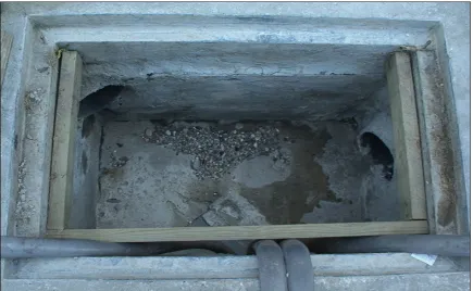
Figure 6. Drainpipes in Manhole from which the Highway Runoff is Collected...82

Figure 7. Example Diagram with Wavelength and Intensity of Al ...90

Figure 8. Flow-Intensity Diagram for all Storm Events...113

Figure 9. Low Flow Intensity Diagram ...114

Figure 10. High Flow Intensity Diagram...114

Figure 11. Accumulative Runoff Flow Diagram for all Storm Events ...115

Figure 12. Accumulative Runoff Flow Diagram for Low Flow Storm Events...116

Figure 13. Accumulative Runoff Flow Diagram for High Flow Storm Events...116

(10)

ix

Figure 15. Average Percentile Concentration of Total Mass Load for

Dissolved Heavy Metal: High Flow Storm Events...119

Figure 16. Average Percentile Concentration of Total Mass Load for

Dissolved Heavy Metal: Low Flow Storm Events ...120

Figure 17. Cumulative Percentage of Al Mass Loading versus Cumulative

Percentage of Discharged Runoff Volume ...123

Figure 18. Cumulative Percentage of Cr Mass Loading versus Cumulative

Figure 19. Cumulative Percentage of Mn Mass Loading versus Cumulative

Figure 20. Cumulative Percentage of Fe Mass Loading versus Cumulative

Figure 21. Cumulative Percentage of Cu Mass Loading versus Cumulative

Figure 22. Cumulative Percentage of Zn Mass Loading versus Cumulative

Figure 23. Cumulative Percentage of Ni Mass Loading versus Cumulative

Figure 24. Mean Cumulative Percentage of Dissolved Heavy Metal Mass

Loading versus Cumulative Percentage of Discharged Runoff Volume.128

Figure 25. Differences in the R Values for the Different Categories...131

Figure 26. Differences in the R² Values for the Different Categories...131

(11)

x

Figure 28. Ln of Predicted vs. Observed Values: Multiple Regression for Ln(Cr )...139

Figure 29. Mean Dissolved Heavy Metal Concentrations for Manganese...141

Figure 30. Ln of Predicted vs. Observed Values: Multiple Regression for Ln(Mn)..142

Figure 31. Predicted vs. Observed Values: Multiple Regression for Fe ...144

Figure 32. Predicted vs. Observed Values: Multiple Regression for Ni ...146

Figure 33. Mean Dissolved Heavy Metal Concentrations: High Flow

vs. Low Flow ...147

Figure 34. Predicted vs. Observed Values: Multiple Regression for Cu ...148

Figure 35. Predicted vs. Observed Values: Multiple Regression for Zn...149

Table 36. Mean Cumulative Percentage of Dissolved Heavy Metal Mass

(12)

xi

LIST OF TABLES

Table 1. Secondary Treatment Standards ...23

Table 2. Typical Components in Untreated Domestic Wastewater...24

Table 3. Discharge Limits for Selected Heavy Metals in Freshwater and Marine Environments. Limits are based on Total Metal Concentrations...36

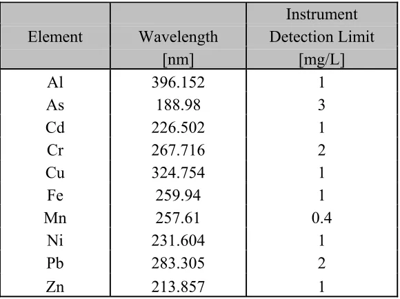
Table 4. Wavelengths used for each Dissolved Heavy Metal Element ...46

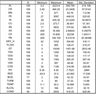
Table 5. Descriptive Statistics: List of Variables and Units ... 93+94 Table 6. Basic Descriptive Statistics of Database...95

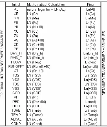
Table 7. Mathematical Procedure for Transformation of Variables ...97

Table 8. Correlation Matrix for all Variables: Untransformed Raw Data Set ...98

Table 9. Correlation Matrix for all Variables: Transformed Raw Data Set...99

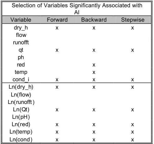
Table 10. Selection of Variables Significantly Associated with Al...102

Table 11. Selection of Variables Significantly Associated with Cr...102

Table 12. Selection of Variables Significantly Associated with Mn ...103

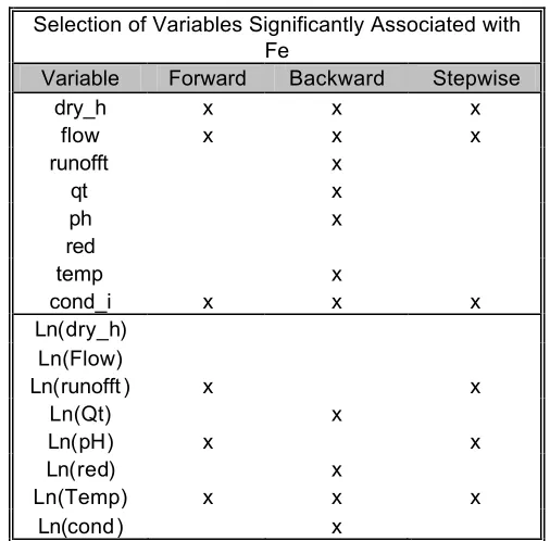
Table 13. Selection of Variables Significantly Associated with Fe...103

Table 14. Selection of Variables Significantly Associated with Ni...104

Table 15. Selection of Variables Significantly Associated with Cu...104

(13)

xii

Table 17. Basic Statistical Values for the Mass Loading of Dissolved Heavy

Metals...118

Table 18. Characterization of Low Flow and High Flow Storm Events...121

Table 19. Primary Sources of Heavy Metal Contamination ...122

Table 20. R and R² Values for the Model Development for Dissolved Heavy Metals...129

Table 21. R and R² Values for the Best Possible Model for Dissolved Heavy Metals...130

Table 22. Differences in the R Values for the Different Categories...131

Table 23. Differences in the R² Values for the Different Categories...131

Table 24. Model Verification for the Entire Dataset (A)...151

Table 25. Model Verification for the Entire Dataset (B) ...151

Table 26. Model Verification for the Entire Dataset: Recalculated...152

(14)

xiii

LIST OF ABBREVIATIONS

x _Mean_of_the_variable

@ at

µmhos/cm Micromhos per centimeter

µs/cm Microsiemens per centimeter

A.D. Ante diem

amu Atomic Mass Units

APHA American Public Health Association

As Arsenic

BCT Best Conventional Pollutant Control Technology

BMPs Best Management Practices

BOD Biochemical Oxygen Demand

BPJ Best Professional Judgment

BPT Best Practicable Control Technology

C° Degrees Celsius

Cd Cadmium

CFR Ciffre

COD Chemical Oxygen Demand

(15)

xiv

Cr Chromium

CSOs Combined Sewer Overflows

Cu Copper

CWA Clean Water Act

D.I. Diplom Ingenieur

DO Dissolved Oxygen

ELGs Effluent Limitations Guidelines

EPA Environmental Protection Agency

F° Fahrenheit

Fe Iron

Hg Mercury

ICP Inductively Coupled Plasma

ICP-OES Inductively Coupled Plasma-Optical Emission Spectrometer

K Kelvin

LSU Louisiana State University

Mn Manganese

MS4s Municipal Separate Storm Sewer Systems

mV Millivolts

Ni Nickel

NPDES National Pollutant Discharge Elimination System

NPS Nonpoint source

Pb Lead

(16)

xv

POTWs Publicly Owned Treatment Works

S Standard Deviation

SSOs Sanitary Sewer Overflows

TDS Total Dissolved Solids

TMDLs Total Maximum Daily Loads

TSS Total Suspended Solids

UNO University of New Orleans

USA United States of America

U.S.EPA United State Environmental Protection Agency

VDS Volatile Dissolved Solids

VSS Volatile Suspended Solids

WLA Waste Load Allocation

(17)

xvi

ABSTRACT

This proposed research focused on the prediction and identification of dissolved

heavy metals in storm water runoff from elevated roadways. Storm water runoff from

highways transports a significant load of contaminants, especially heavy metals and

particulate matter, to receiving waters. Heavy metals, either in dissolved or

particulate-bound phases, are unique in the fact that unlike organic compounds, they are not

degraded in the environment.

The objective of this research was to develop a mathematical model to relate

dissolved heavy metal concentration to different measurable parameters which are easily

available and routinely measurable for elevated roadways. The reliability of the

developed models was then evaluated by comparing the raw data versus data predicted by

the models.

The test site for this research was selected at the intersection of the Interstate-10

and Interstate-610, Orleans Parish, New Orleans, Louisiana. Subsequently a research test

site was developed and highway storm water runoff was collected. Volumetric flow rates

were measured with every collected sample by measuring the amount of collected water

and the collection time. Storm water runoff from the examined elevated roadway section

was sampled for 10 storm events throughout the course of the study from which

(18)

xvii

The measurement of different parameters made it possible to determine the

percentage of dissolved heavy metal mass loading and the characterization of high runoff

flow intensity and low runoff flow intensity storm events.

Another very important achievement in this research was the construction of a

predictive model for dissolved heavy metal concentrations based on field measurements.

Data analysis proceeded by applying different variable selection statistical methods as

well as multiple regression analyses in order to evaluate the simultaneous effects of all

variables on the concentration of dissolved heavy metals in storm water runoff. The

developed model enables the user to predict dissolved heavy metal concentrations with

known field measurements within a prediction interval of 95 % confidence.

The reliability of the models was verified by carrying out significant-difference

(19)

CHAPTER 1 INTRODUCTION

Anthropogenic constituents in highway runoff include metal elements and

suspended solids which result from traffic activities, atmospheric deposition, roadway

degradation and highway maintenance. Storm water runoff from urban areas transports

significant loads of heavy metals, a wide gradation of particulate matter, dissolved solids,

organic compounds and inorganic constituents. Heavy metals are not degraded in the

environment and constitute an important class of contaminants generated through modern

urban activities and infrastructure. In urban areas one major source of heavy metals are

traffic activities. In urban runoff discharges levels of Zn, Cu, Cd, Pb, Cr and Ni are

significantly above ambient background levels, and for many urban areas, Zn, Cu, and Cd

often exceed United State Environmental Protection Agency(U.S.EPA)and State EPA

surface water discharge criteria on an event basis. Treatment of storm water continues to

pose unique challenges due to unsteady nature of processes including rainfall-runoff,

mobilization and transport of heavy metal as well as other constituent loads. Additionally,

kinetics of heavy metal partitioning as a function of pH, residence time and particulate

matter characteristics can have a profound effect on the selection and effectiveness of

(20)

The enormous demands being placed on water supply and wastewater disposal

facilities today have necessitated the development and implementation of far broader

concepts in environmental engineering than those envisioned only a few years ago. The

regulations and standards for water quality have significantly increased concurrently with

a decrease in water quality. Evidence of water supply contamination by toxic and

hazardous materials has become common and concern about broad water-related

environmental issues has heightened. As populations throughout the world multiply at an

alarming rate, environmental control and water management become increasingly urgent.

(Viessman, 1998)

During the past century, large areas were filled with urban construction to create

business and residential centers and to enhance human lifestyle. Infrastructures such as

roadway pavements, parking lots, rooftops, sidewalks and driveways were built in order

to improve people’s mobility and quality of life. These pavement surfaces are highly

impervious in nature and were designed for a rapid and efficient transport of storm water

flows. This higher hydraulic efficiency enhances the amount and velocity of urban storm

water runoff and consequently promotes the pollutant transport from infrastructures.

A consequence of the growing population densities in many areas of the world is

increasing traffic and the associated traffic-generated pollution. Increasing traffic causes

a rise in the amount of contaminants accumulating on road surfaces which results in

higher concentrations of contaminants and contaminant loads transported off the

impermeable infrastructures into receiving waters.

Storm water runoff from highways transports a significant load of contaminants,

(21)

in dissolved or particulate-bound phases, are unique in the fact that unlike organic

compounds, they are not degraded in the environment. Because of their short- and

long-term toxic effects, the maximum permissible concentrations of these heavy metals in

drinking water as well as in municipal and industrial discharges are closely regulated

through legislation. (SenGupta, 2002)

The U.S. EPA issued a policy memorandum on October 1, 1993, which was

titled “Office of Water Policy and Technical Guidance on Interpretation and

Implementation of Aquatic Metals Policy” and stated:

“It is now the policy of the Office of Water that the use of dissolved metal to set

and measure compliance with water quality standards is the recommended approach,

because dissolved metal more closely approximates the bio-available fraction of metal in

the water column than does total recoverable metal”. Therefore this research can be

useful, especially for non point sources, to assess and predict dissolved heavy metals in

storm water runoff from roadways and similar. (U.S. EPA, 1996b)

A better understanding of dissolved heavy metals, their concentration and

correlation of storm water runoff is necessary. The goal of this study is therefore to

perform a thorough investigation on storm water runoff from elevated roadways in order

to provide useful results for further research regarding the concentration of dissolved

(22)

CHAPTER 2 SCOPE AND OBJECTIVES

This proposed research focused on storm water runoff from highways. These

runoffs represent a considerable contaminant source for the surrounding receiving waters.

During this study eleven storm events were observed and multiple storm water runoff

samples were collected from each storm event and analyzed for many different

parameters.

The Environmental Protection Agency (EPA) recommends that state water quality

standards should be based on dissolved heavy metal concentrations because the dissolved

fraction is a better representation of the biologically active portion of the metal in water

than is the total or total recoverable fraction. (U.S. EPA, 1996b)

Therefore, this document will focus on dissolved heavy metals and their

correlation with different water parameters in order to create a predictive model for

dissolved heavy metals.

Based on this, the proposed research focuses on three primary objectives:

Objective 1: The first objective of this research was to analyse samples collected from

(23)

methods and to evaluate the data gathered in order to determine the most

important variables affecting highway storm water runoff. (APHA, 1999)

Objective 2: The second objective of this study focused on calculating and evaluating

scatter plots and statistical correlations between several variables such as

pollutant concentrations, runoff volume, traffic flow, antecedent dry

hours, runoff intensity, pH, redox, temperature, runoff time, etc.

Objective 3: The third objective in this research was to construct a mathematical

regression model to predict dissolved heavy metal concentrations in storm

water runoff. The importance of such a model should be emphasized

since the duration of the analyses of highway storm water samples for

many different elements is a considerable time and cost factor. The goal

was to determine storm water parameters that are relatively easy and fast

to analyze and show a strong correlation with dissolved heavy metals.

Especially dissolved heavy metal analyses require an enormous technical

expenditure and expensive laboratory equipment which result in high costs

and time expenses.

The use of this mathematical model makes it possible to predict

dissolved heavy metal concentrations in the storm water runoff from roads

and highways. The achievement of this objective may save considerable

time and money for future rainfall runoff analyses and may consequently

(24)

CHAPTER 3 LITERATURE REVIEW

3.1 The Clean Water Act

In December 1970, as an outgrowth of the administration’s environmental interests, a new independent body, the Environmental Protection Agency (EPA), was created. This organization assumed the functions of several existing agencies relative to matters of environmental management. It brought together under one roof all of the pollution control programs related to water, air, solid wastes, pesticides, and radiation. The EPA was seen by the administration as the most effective way of recognizing that the environment must be looked on as a single, interrelated system. It is noteworthy, however, that the creation of the EPA made even more pronounced the separation of water quality programs from other water programs.

(25)

The act departed in several ways from previous water pollution control legislation. It expanded the federal role in water pollution control, increased the level of federal funding for construction of publicly owned treatment works, elevated planning to a new level of significance, opened new avenues for public participation, and created a regulatory mechanism requiring uniform technology-based effluent standards, together with a national permit system for all point-source dischargers as the means of enforcement. As pollution control measures for industrial process wastewater and municipal sewage were implemented and refined, it became increasingly evident that more diffuse sources of water pollution were also significant causes of water quality impairment. Specifically, storm water runoff draining from large surface areas, such as urban land, was found to be a major cause of water quality impairment, including the non-attainment of designated beneficial uses. (Viessman, et al., 1998)

The Clean Water Act (CWA) is the cornerstone of surface water quality protection in the United States. The Act does not deal directly with ground water or with water quantity issues. The statute employs a variety of regulatory and non-regulatory tools to sharply reduce direct pollutant discharges into waterways, finance municipal wastewater treatment facilities, and manage polluted runoff. These tools are employed to achieve the broader goal of restoring and maintaining the chemical, physical, and biological integrity of the nation's waters.

(26)

discharges from traditional point source facilities, such as municipal sewage plants and industrial facilities, with little attention paid to runoff from streets, construction sites, farms, and other wet-weather sources.

Starting in the late 1980s, efforts to address polluted runoff have increased significantly. For nonpoint runoff, voluntary programs, including cost-sharing with landowners are the key tool. For wet weather point sources like urban storm sewer systems and construction sites, a regulatory approach is being employed. Evolution of CWA programs over the last decade has also included something of a shift from a program-by-program, source-by-source, pollutant-by-pollutant approach to more holistic watershed-based strategies. (U.S. EPA, 2003b)

3.2 Development of the NPDES Storm Water Program

The National Pollutant Discharge Elimination System (NPDES) Storm Water Program has been established with the intention to regulate storm water runoff from point sources through permits. To accomplish these regulations a two phase program was induced. These two different phases will be discussed in the following sections.

3.2.1 Phase I NPDES Storm Water Program

(27)

Phase I of the U.S. Environmental Protection Agency’s (EPA) storm water program was promulgated in 1990 under the CWA. The Phase I program addressed sources of storm water runoff that had the greatest potential to negatively impact water quality. Phase I relies on National Pollutant Discharge Elimination System (NPDES) permit coverage to address storm water runoff from:

• “Medium” and “large” municipal separate storm sewer systems (MS4s)

generally serving populations of 100,000 or greater • Construction activity disturbing 5 acres of land or greater

• Ten categories of industrial activity.

Operators of the facilities, systems, and construction sites regulated under the Phase I NPDES Storm Water Program can obtain permit coverage under an individually tailored NPDES permit or a general NPDES permit. The first permit was developed for MS4 and some industrial facilities, whereas the second permit was used by most operators of industrial facilities and construction sites. (U.S. EPA, 2000)

(U.S. EPA, 1999b)

3.2.2 Phase II NPDES Storm Water Program

(28)

polluted storm water runoff. Phase II is intended to further reduce adverse impacts to water quality and aquatic habitat by instituting the use of controls on the unregulated sources of storm water discharges that have the greatest likelihood of causing continued environmental degradation.

The Phase II regulations established a sequential application process for all Phase II storm water discharges, which included all discharges, composed entirely of storm water, except those specifically classified as Phase I discharges. Such discharges included storm water from small municipal separate storm sewer systems, and commercial and institutional facilities. The application regulations included two tiers. The first tier was for Phase II dischargers, that the NPDES permitting authority determined were contributing to water quality impairment or were a significant contributor of pollutants to waters of the United States. Dischargers that have been designated by the permitting authority were required to obtain a permit and had to submit a permit application within 180 days of notification that an application was required. The second tier of the Phase II storm water application regulations required all remaining Phase II sources (i.e., all Phase II sources not designated by the permitting authority) to submit a permit application by August 7, 2001, but only if the Phase II regulatory Program in place at that time required permits.

Three new classes of facilities were designated for automatic coverage on a nationwide basis:

• Operators of small municipal separate storm sewer

systems (MS4s) serving population centers (or

(29)

population density of 1,000 people per square mile. (about 3500 municipalities)

• Construction activity disturbing between 1 and 5 acres of land,

such as small construction activities.

• All highways and streets discharging to MS4s

In addition to expanding the NPDES Storm Water Program, the Phase II Final Rule revises the "no exposure" exclusion and the temporary exemption for certain industrial facilities under Phase I of the NPDES Storm Water Program. (U.S. EPA, Office of Water, January 2000)

3.2.3 Wet Weather Discharges

(30)

quality, reduce redundant contamination control costs, and provide State and local governments with greater flexibility to solve wet weather discharge problems. To identify and address cross-cutting issues and promote coordination, EPA established the Urban Wet Weather Flows Federal Advisory Committee in 1995.

(U.S. EPA, 1995a”)

3.3 Contaminant Sources and their Effects

In this section some background information on storm water runoff from highways will be discussed. Furthermore, definitions and explanations of the most important aspects of the special topic of storm water runoff from elevated highways will be provided.

3.3.1 Distinction between Non-Point- and Point-Sources

Since there is often a misunderstanding in the meaning of non-point and point sources a definition is given in the following section.

3.3.1.1 Point Sources

(31)

types of ships, tank trucks, offshore oil platforms, and collected runoff from many construction sites. (U.S. EPA, 2003a)

3.3.1.2 Non-Point sources

Nonpoint source (NPS) pollution, unlike pollution from industrial and sewage treatment plants, comes from many diffuse sources. NPS pollution is caused by rainfall or snowmelt moving over and through the ground. As the runoff moves, it picks up and carries away natural and human-made pollutants, finally depositing them into lakes, rivers, wetlands, coastal waters, and even our underground sources of drinking water. Loadings of pollutants from NPS enter water-bodies via sheet flow, rather than through a pipe, ditch or other conveyance.

These pollutants include:

• Excess fertilizers, herbicides, and insecticides from agricultural lands and

residential areas;

• Oil, grease, and toxic chemicals from urban runoff and energy production; • Sediment from improperly managed construction sites, crop and forest lands,

and eroding stream-banks;

• Salt from irrigation practices and acid drainage from abandoned mines;

• Bacteria and nutrients from livestock, pet wastes, and faulty septic systems;

Atmospheric deposition and hydro-modification are also sources of nonpoint source pollution.

(32)

and may not always be fully assessed. However, we know that these pollutants have harmful effects on drinking water supplies, recreation, fisheries, and wildlife.

Other impacts associated with urbanization are the increasing amount of storm water runoff, contribution to stream bank erosion and possibility of downstream flooding. Impervious concrete and asphalt surfaces of new roadways prevent storm water from soaking into the ground, where it was once absorbed. This increases the total volume of storm water runoff. It also increases the value of the peak storm water discharge, and decreases the time it takes to reach this peak. Increased runoff volumes and peak discharge levels result in increased levels of flooding risk.

Collecting runoff water from non-point sources, such as roadway shoulders, is difficult, thus in this research project, storm water runoff from an elevated highway has been analyzed. Samples were collected from the drainage pipe of this elevated highway, which collects water from a known impervious area. Consequently, calculating the volume of the storm water runoff and addressing the contaminant loading to this known area was possible. (U.S. EPA, 2002b) (U.S. EPA, 2003a)

3.3.2 Factors affecting Runoff Quality

(33)

3.3.2.1 Sources

One of the major contaminant sources of storm water runoff is traffic. All means of transportation directly and indirectly contribute much to the contamination found in highway runoff. Vehicles are a source of metals, oil, grease, lead, asbestos, and rubber. Sometimes de-icing chemicals such as salts or other materials deposited on highways are also indirectly contributed to vehicles. Other major sources of contaminants in the runoff include dust that settles on the road and shoulders and dissolved constituents, such as acids and particulate matter from atmospheric fallout. Urban construction sites contribute sediment, plant debris, and asphalt. Storm water runoff also contains refuse such as street litter. A number of common highway maintenance practices, such as salting, also may adversely affect water quality. The nature of the materials, methods used, and the proximity of the maintenance activity to a body of water increase the likelihood of adverse effects. (Schöpf, R., August 2002)

3.3.2.2 Highway Runoff Quality

(34)

associated with particulate matter, such as dust, which are more easily mobilized in high intensity storms. Constituents in storm water runoff showing a strong correlation with suspended solids include metals, organic compounds, total organic carbon, and biochemical oxygen demand.

Higher concentrations of contaminants are often observed in the first runoff from a storm, a phenomenon referred to as first flush effect. This is especially true for dissolved components including nutrients, organic lead, and ionic constituents.

In general, concentrations of particle-associated contaminants show a more complex temporal variation related to rainfall intensity and the flushing of sediment through the drainage system.

The effect of highway paving material (asphalt versus concrete) on the quality of highway runoff appears to be minimal. Most studies have found that highway surface type was relatively unimportant compared to such factors as surrounding land use. It has also been reported that the type of collection and conveyance system for highway runoff, such as storm sewer, grassy swale has a greater effect on runoff quality than pavement type. (Department of Environmental Resources, 2003)

3.3.2.3 Contaminants in Runoff Pollution

(35)

Runoff pollution is that associated with rainwater or melting snow that washes off roads, bridges, parking lots, rooftops, and other impermeable surfaces. As it flows over these surfaces, the water picks up dirt and dust, rubber and metal deposits from tire wear, antifreeze and engine oil that has dripped onto the pavement, pesticides and fertilizers, and discarded cups, plastic bags, cigarette butts, pet waste, and other litter. These contaminants are carried into our lakes, rivers, streams, and oceans.

Contaminants in runoff pollution from roads, highways, and bridges include:

Sediment:It is mainly produced when soil particles are eroded from the land and transported to surface waters. Natural erosion usually occurs gradually because vegetation protects the ground. When land is cleared or disturbed to build a road or bridge, however, the rate of erosion increases. The vegetation is removed and the soil is left exposed, to be quickly washed away in the next rain. Erosion around bridge structures, road pavements, and drainage ditches can damage and weaken these structures.

Soil particles settle out of the water in a lake, stream, or bay onto aquatic plants, rocks, and the bottom. This sediment prevents sunlight from reaching aquatic plants, clogs fish gills, chokes other organisms, and can smother fish spawning and nursery areas.

(36)

Oils and Grease: Oils and grease are leaked onto road surfaces from car and truck engines, spilled at fueling stations, and discarded directly onto pavement or into storm sewers instead of being taken to recycling stations. Rain and snowmelt transport these pollutants directly to surface waters.

Heavy Metals: Heavy metals come from some "natural" sources such as minerals in rocks, vegetation, sand, and salt. But they also come from car and truck exhaust, worn tires and engine parts, brake linings, weathered paint, and rust. Heavy metals are toxic to aquatic life and can potentially contaminate ground water.

Debris: Grass and shrub clippings, pet waste, food containers, and other household wastes and litter can lead to unsightly and polluted waters. Pet waste from urban areas can add enough nutrients to estuaries to cause premature aging, or "eutrophication."

Road Salts: In the snowbelt, road salts can be a major pollutant in both urban and rural areas. Snow runoff containing salt can produce high sodium and chloride concentrations in ponds, lakes, and bays. This can cause unnecessary fish kills and changes to water chemistry.

(37)

3.3.2.4 Effects of Highway Runoff

The type and size of the receiving body, the potential for dispersion, the size of the catchment’s area, the relative amount of highway runoff, and the biological diversity of the receiving water ecosystem are just some of the factors that determine the extent and importance of highway runoff effects. Concentrations of contaminants in the water columns of receiving waters generally show small changes due to highway runoff. This may be the result of dilution of the highway runoff by flow from the rest of the watershed. However, stream and lake sediments have been found to have high concentrations of heavy metals and are the primary source for the bioconcentration of metals in aquatic biota.

Bioassay tests of organisms from streams and lakes receiving highway runoff generally have not demonstrated acute toxicity, although very high traffic volumes or other site-specific conditions may produce a toxic response. Chronic toxicity resulting from bioaccumulation of contaminants in highway runoff has not been thoroughly investigated, although studies have documented higher concentrations of metals in fish and other aquatic biota living near highways (Department of Environmental Resources, 2003).

(38)

groundwater through retention, modification, decomposition, or adsorption. Therefore, groundwater contamination is a particular concern where the aquifer is shallow (less than 4 feet). (U.S. EPA, Office of Water, August 1995, 12.04.2003)

3.4 NPDES Effluent Limits

When developing effluent limits for a NPDES permit, a permit writer must consider limits based on both the technology available to treat the pollutants (i.e., technology-based effluent limits), and limits that are protective of the water quality standards of the receiving water (i.e., water quality-based effluent limits). (U.S. EPA, April 1996a )

3.4.1 Quality-based Effluent Limits

(39)

approach uses best management practices (BMPs) in first-round storm water permits, and expanded or better-tailored BMPs in subsequent permits, where necessary, to provide for the attainment of water quality standards. In cases where adequate information exists to develop more specific conditions or limitations to meet water quality standards, these conditions or limitations are to be incorporated into storm water permits, as necessary and appropriate. This interim permitting approach is not intended to affect those storm water permits that already include appropriately derived numeric water quality-based effluent limitations. Since the policy only applies to water quality based effluent limitations, it is not intended to affect technology-based limitations, such as those based on effluent guidelines or the permit writer’s best professional judgment, that are incorporated into storm water permits.

Each storm water permit should include a coordinated and cost-effective monitoring program to gather necessary information to determine the extent to which the permit provides for attainment of applicable water quality standards and to determine the appropriate conditions or limitations for subsequent permits. Such a monitoring program may include ambient monitoring, receiving water assessment, discharge monitoring (as needed), or a combination of monitoring procedures designed to gather necessary information.

(40)

Urban Wet Weather Flows Federal Advisory Committee policy dialogue on this subject. (U.S. EPA, 2003c) (lity-Based Permitting”) (U.S.EPA, 2003e)

3.4.2 Technology-based Effluent Limits

There are two general approaches for developing technology-based effluent limits for industrial facilities:

1. Using National Effluent Limitations Guidelines (ELGs) and

2.Using Best Professional Judgment (BPJ) on a case-by-case basis (in the absence of ELGs).

3.4.2.1 National Effluent Limitation Guideline (ELGs)

(41)

and BPJ (as well as water quality considerations) may be included in a single permit. When developing technology-based effluent limitations for non-municipal dischargers, the permit writer must consider all applicable standards and requirements for all pollutants discharged. As indicated above, applicable technology-based requirements may include national standards and requirements applicable to all facilities in specified industrial categories, or facility-specific technology-based requirements based on the permit writer’s BPJ. It is important, therefore, that permit writers understand the basis of the national standards and the differences between the various required levels of treatment performance.

An important aspect of municipal wastewater is that it is amenable to biological treatment. The biological treatment component of a municipal treatment plant is termed secondary treatment and is usually preceded by simple settling (primary treatment). In response to the CWA requirements, EPA evaluated performance data for POTWs practicing secondary treatment and established performance standards based on its evaluation. Secondary treatment standards, therefore, are defined by the limitations provided in Table 1.

Parameter 30-Day Average 7-Day Average

5-Day BOD 30mg/l 45mg/l

TSS 30mg/l 45mg/l

pH 6 – 9 s.u. (instantaneous) ---

Removal 85% BOD5 and TSS ---

(42)

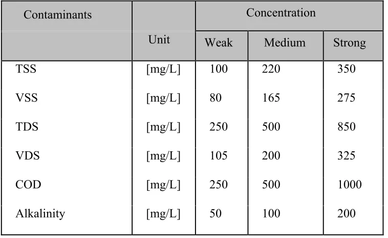
Table 2 shows typical concentrations which can be found in untreated domestic

wastewater.

Contaminants Concentration

Unit _Weak _Medium _Strong

TSS [mg/L] 100 220 350

VSS [mg/L] 80 165 275

TDS [mg/L] 250 500 850

VDS [mg/L] 105 200 325

COD [mg/L] 250 500 1000

Alkalinity [mg/L] 50 100 200

Table 2: Typical Components in Untreated Domestic Wastewater (U.S. EPA, 2001,

“Water Quality-Based Permitting”, 2003)

Effluent limitations guidelines and performance standards are established by EPA

for different industrial categories since the best control technology for one industry is not

necessarily the best for another. These guidelines are developed based on the degree of

pollutant reduction attainable by an industrial category through the application of control

technologies, irrespective of the facility location. Using these factors, similar facilities

are regulated in the same manner. In theory, for example, a pulp and paper mill on the

west coast of the United States would be required to meet the same technology-based

(43)

site-specific concerns that had to be addressed). To date, EPA has established guidelines and standards for more than 50 different industrial categories (e.g., metal finishing facilities, steam electric power plants, iron and steel manufacturing facilities). (U.S. EPA, 2001, ) (U.S.EPA, 2003e) (U.S.EPA, 1996a) (U.S. EPA, 2003c)

3.4.2.2 Best Professional Judgment (BPJ) Limits

Best Professional Judgment limits (BPJ-based limits) are technology-based limits derived on a case-by-case basis for non-municipal (industrial) facilities. BPJ limits are established in cases where ELGs are not available for, or do not regulate, a particular pollutant of concern. BPJ is defined as the highest quality technical opinion developed by a permit writer after consideration of all reasonably available and pertinent data or information that forms the basis for the terms and conditions of a NPDES permit. The authority for BPJ is contained in Section 402(a)(1) of the CWA, which authorizes the EPA Administrator to issue a permit containing “such conditions as the Administrator determines are necessary to carry out the provisions of this Act”, prior to taking the necessary implementing actions, such as the establishment of ELGs.

(44)

permit writers had to rely less on their best engineering judgment and could apply the ELGs in permits. As the implementation of the age of toxic pollutant control continues, the use of BPJ conditions in permits has again become more common. However, the statutory deadline for compliance with technology-based effluent limits (including BPJ-based pollutant limits) was March 31, 1989. Therefore, compliance schedules cannot be placed in permits to allow for extensions in meeting BPJ pollutant limits. BPJ has proven to be a valuable tool for NPDES permit writers over the years. Because it is so broad in scope, BPJ allows the permit writer considerable flexibility in establishing permit terms and conditions. Inherent in this flexibility, however, is the burden on the permit writer to show that the BPJ is reasonable and based on sound engineering analysis. If this evaluation of reasonableness does not exist, the BPJ condition is vulnerable to a challenge by the permittee. Therefore, the need for and derivation of the permit condition, and the basis for its establishment, should be clearly defined and documented. References used to determine the BPJ condition should be identified. In short, the rationale for a BPJ permit must be carefully drafted to withstand the scrutiny of not only the permittee, but also the public and, ultimately, an administrative law judge. (U.S. EPA, April 1996 a)

3.4.2.3 Establishment of BPJ Permit Limits

(45)

• The appropriate technology for the category class of point sources of which the

applicant is a member, based on all available information, and • Any unique factors relating to the applicant.

To set BPJ limits, a permit writer must first determine a need for additional controls beyond existing ELGs. The need for additional controls may be the result of the facility not falling under any of the categories for which ELGs exist (e.g., barrel reclaimers, transportation equipment cleaning facilities, or industrial laundries) or discharging pollutants of concern that are not directly or indirectly addressed by the development of the ELGs (e.g., a pharmaceutical manufacturer or a petroleum refiner may discharge elevated levels of organic solvents for which category-specific guidelines do not exist). It should be noted that prior to establishing BPJ-based limits for a pollutant not regulated in an effluent guideline, the permit writer should ensure that the pollutant was not considered by EPA while developing the ELGs (i.e., BPJ based effluent limits are not required for pollutants that were considered by EPA for regulation under the effluent guidelines, but for which EPA determined that no ELG was necessary).

In setting BPJ limitations, the permit writer must consider several specific factors as they appear in 40 CFR §125.3(d). These factors, which are enumerated below, are the same factors required to be considered by EPA in the development of ELGs and, therefore, are often referred to as the Section 304(b) factors:

• For best practicable control technology (BPT) requirements:

(46)

– The age of equipment and facilities involved – The process employed

– The engineering aspects of the application of various types of control techniques

– Process changes*

– Non-water quality environmental impact including energy requirements* • For best conventional pollutant control technology (BCT) requirements:

– All items in the (BPT) requirements indicated by an asterisk (*) above – The reasonableness of the relationship between the costs of attaining a

reduction in effluent and the effluent reduction benefits derived

– The comparison of the cost and level of reduction of such pollutants from the discharge of POTWs to the cost and level of reduction of such pollutants from a class or category of industrial sources

• For best available technology (BAT) requirements:

– All items in the BPT requirements indicated – The cost of achieving such effluent reduction.

(47)

with existing technology. “Reasonable” means that the conditions are achievable at a cost that the facility can afford. Historically, some of the other factors, such as age, process employed and non-water quality impacts have assumed lesser importance than the technical and economic feasibility evaluations.

(U.S. EPA, April 1996a)

3.5 Total Maximum Daily Loads (TMDLs)

Over 40 % of United States waters still do not meet the water quality standards states, territories, and authorized tribes have set for them. This amounts to over 20,000 individual river segments, lakes, and estuaries. These impaired waters include approximately 300,000 miles of rivers and shorelines and approximately 5 million acres of lakes - polluted mostly by sediments, excess nutrients, and harmful microorganisms. An overwhelming majority of the population (218 million) lives within 10 miles of the impaired waters.

Under section 303(d) of the 1972 Clean Water Act, states, territories, and authorized tribes are required to develop lists of impaired waters. These impaired waters do not meet water quality standards that states, territories, and authorized tribes have set for them, even after point sources of pollution have installed the minimum required levels of pollution control technology. The law requires that these jurisdictions establish priority rankings for waters on the lists and develop TMDLs for these waters.

(48)

and TMDLs established by states, territories, and authorized tribes. If a state, territory, or authorized tribe submission is inadequate, EPA must establish the list or the TMDL. EPA issued regulations in 1985 and 1992 that implement section 303(d) of the Clean Water Act - the TMDL provisions.

In an effort to speed the Nation's progress toward achieving water quality standards and improving the TMDL program, EPA began, in 1996, a comprehensive evaluation of EPA's and the states' implementation of their Clean Water Act section 303(d) responsibilities. EPA convened a committee under the Federal Advisory Committee Act, composed of 20 individuals with diverse backgrounds, including agriculture, forestry, environmental advocacy, industry, and state, local, and tribal governments. The committee issued its recommendations in 1998.

These recommendations were used to guide the development of proposed changes to the TMDL regulations, which EPA issued in draft in August 1999. After a long comment period, hundreds of meetings and conference calls, much debate, and the Agency's review and serious consideration of over 34,000 comments, the final rule was published on July 13, 2000. However, Congress added a "rider" to one of their appropriations bills that prohibits EPA from spending “FY2000” and “FY2001” money to implement this new rule.

(49)

tribes list impaired and threatened waters and develop TMDLs.

(U.S. EPA, 2002a)

3.6 _{Best Management Practice}

Best Management Practices (BMP) can be either structural or non-structural practices that are implemented to minimize the impacts of anthropogenic constituents

generated by urban and traffic activities on water quality. The term was first used in the

(50)

3.6.1 Types of Storm Water BMPs

There are a variety of storm water BMPs available for managing urban runoff. Regardless of the type, storm water BMPs are most effective when implemented as part of a comprehensive storm water management program that includes proper selection, design, construction, inspection and maintenance. Storm water BMPs can be grouped into two broad categories: structural and non-structural. Structural BMPs are used to treat the storm water at either the point of generation or the point of discharge to either the storm sewer system or to receiving waters. Non-structural BMPs include a range of pollution prevention, education, institutional, management and development practices designed to limit the conversion of rainfall to runoff and to prevent pollutants from entering runoff at the source of runoff generation.

(U.S. EPA, 1999a)

3.6.2 BMP Selection

(51)

new land development, where opportunities exist for incorporating BMPs that are focused on runoff prevention, reducing impervious surfaces and maintaining natural drainage patterns. In established urban communities, a different suite of BMPs may be more appropriate due to space constraints. In these areas, BMPs may be selected to focus on pollution prevention practices along with retrofit of the established storm drain system with regional BMPs. Site suitability for selecting a particular BMP strategy is key to successful performance. Most BMPs have limitations for their applicability, and therefore cannot be applied nationwide.

(U.S. EPA, 1999a)

3.6.3 Effectiveness of BMPs

(52)

structural BMPs. (U.S. EPA, 1999, “Description and Performance of Storm Water Best Management Practices”, Urban Storm Water BMP Study)

3.7 Heavy Metals

Heavy metals are elements having atomic weights between 63.546 and 200.590, and a specific gravity greater than 4.0. Living organisms require trace amounts of some heavy metals, including cobalt, copper, iron, manganese, molybdenum, vanadium, strontium, and zinc. Excessive levels of essential metals, however, can be detrimental to the organism. Non-essential heavy metals of particular concern to surface water systems are cadmium, chromium, mercury, lead, arsenic, and antimony.

All heavy metals exist in surface waters in colloidal, particulate, and dissolved phases, although dissolved concentrations are generally low. The colloidal and particulate metal may be found in

1) Hydroxides, oxides, silicates, or sulfides; or 2) Adsorbed to clay, silica, or organic matter.

The soluble forms are generally ions or unionized organometallic chelates or complexes. The solubility of trace metals in surface waters is predominately controlled by the water pH, the type and concentration of ligands on which the metal could adsorb, and the oxidation state of the mineral components and the redox environment of the system.

(53)

composed of fine sand and silt will generally have higher levels of adsorbed metal than will quartz, feldspar, and detrital carbonate-rich sediment. Metals also have a high affinity for humic acids, organo-clays, and oxides coated with organic matter.

The water chemistry of the system controls the rate of adsorption and desorbtion of metals to and from sediment. Adsorption removes the metal from the water column and stores the metal in the substrate. Desorption returns the metal to the water column, where recirculation and bioassimilation may take place. Metals may be desorbed from the sediment if the water experiences increases in salinity, decreases in redox potential, or decreases in pH.

1. Salinity increase: Elevated salt concentrations create increased

competition between cations and metals for binding sites. Often, metals will be driven off into the overlying water. (Estuaries are prone to this phenomenon because of fluctuating river flow inputs.)

2. Redox Potential decrease: A decreased redox potential, as is often seen under oxygen deficient conditions, will change the composition of metal complexes and release the metal ions into the overlying water.

(54)

Heavy metals in surface water systems can be from natural or anthropogenic sources. Currently, anthropogenic inputs of metals exceed natural inputs. Excess metal levels in surface water may pose a health risk to humans and to the environment.

Although living organisms require trace amounts of some heavy metals, including cobalt, copper, iron, manganese, molybdenum, vanadium, strontium, and zinc, excessive levels, however, can be detrimental. (Water Quality Group, “Heavy Metals in Watersheds”, 2003)

Table 3. Discharge Limits for Selected Heavy Metals in Freshwater and Marine

Environments. Limits are based on Total Metal Concentrations (Dissolved and Particulate) and a Hardness of 100-mg/L (U.S.EPA 1999). (ASCE (Dean et al.) 19 May 2003)

3.7.1 Aluminum

Basic Information

Name: Aluminum Symbol: Al

(55)

Atomic Mass: 26.981539 amu

Melting Point: 660.37 °C (933.52 °K, 1220.666 °F) Boiling Point: 2467.0 °C (2740.15 °K, 4472.6 °F) Number of Protons/Electrons: 13

Number of Neutrons: 14 Classification: Other Metals Crystal Structure: Cubic Density @ 293 K: 2.702 g/cm3 Color: Silver

British Spelling: Aluminium IUPAC Spelling: Aluminium

Atomic Structure

Number of Energy Levels: 3 First Energy Level: 2

(56)

Isotopes

Isotope Half Life

Al-26 730000.0 years

Al-27 Stable

Al-28 2.3 minutes

Facts

Date of Discovery: 1825

Discoverer: Hans Christian Oersted

Name Origin: From the Latin word alumen

Uses: As the pure metal or as alloys (magnalium, aluminum bronze, etc.) for

aircraft, utensils, apparatus, electrical conductors; instead of copper in dental

alloys. The coarse powder is used in aluminothermics (thermite process); the fine

powder as flashlight in Photography, in explosives, fireworks and in aluminum

paints; for absorbing occluded gases in manufactories of steel. In testing for Au,

As, Hg; coagulating colloidal solution. of As or Sb; reducer for determining

nitrates and nitrites; instead of Zn for generating hydrogen in testing for As.

Aluminum toxicity has been recognized in many settings where exposure is heavy

(57)

burden is released in stress or illness. Toxicity may include: encephalopathy (stuttering, gait disturbance, myoclonic jerks, seizures, coma, abnormal EEG) osteomalacia or aplastic bone disease ( associated with painful spontaneous fractures, hypercalcemia, tumorous calcinosis ) proximal myopathy, increased risk of infection, increased left ventricular mass and decreased myocardial function microcytic anemia with very high levels, sudden death.

Aluminum is ubiquitous in our environment; it is the third most prevalent element in the earth's crust. The gastrointestinal tract is relatively impervious to aluminum, absorption normally being only about 2%. Aluminum is absorbed by a mechanism related to that for calcium. Gastric acidity and oral citrate favors absorption, and H2-blockers reduce absorption. As is true for several trace elements, transferrin is the primary protein binder and carrier for aluminum in the plasma, where 80% is protein bound and 20% is free or complexed to small molecules such as citrate.

(58)

3.7.2 Arsenic

Basic Information

Name: Arsenic Symbol: As

Atomic Number: 33

Number of Neutrons: 42 Classification: Metalloid

Crystal Structure: Rhombohedral Density @ 293 K: 5.72 g/cm3 Color: Gray

Atomic Structure

(59)

Isotopes

Isotope Half Life As-71 2.7 days As-72 26.0 hours As-73 80.3 days As-74 17.8 days As-75 Stable As-76 26.3 hours As-77 39.0 hours As-79 9.0 minutes

Facts

Date of Discovery: Known to the ancients Discoverer: Unknown

Name Origin: From the Greek word arsenikos and the Latin word arsenicum

Uses: Poison, conducts electricity, semiconductors

(60)

natural sources was linked to skin cancer. When discussing arsenic, speciation plays an especially important role: hydrides, halogenides, oxides, sulfides, arsenites, arsenates, and organic arsenic compounds all have very different properties (i.e., arsenic trihydride is a colorless, extremely poisonous neutral gas). (Merian, E., 1991)

Arsenic ingestion can cause severe toxicity through ingestion of contaminated food and water. Ingestion causes vomiting, diarrhea and cardiac abnormalities. (Water Quality Group, 05.13.2002) (Yinin Bentor, 11.13.2003)

3.7.3 Cadmium

Basic Information

Name: Cadmium Symbol: Cd

(61)

Atomic Structure

Number of Energy Levels: 5 First Energy Level: 2 Second Energy Level: 8 Third Energy Level: 18 Fourth Energy Level: 18 Fifth Energy Level: 2

Isotopes

Isotope Half Life Cd-106 Stable Cd-108 Stable Cd-109 462.0 days Cd-110 Stable Cd-111 Stable Cd-111m 48.5 minutes Cd-112 Stable Cd-113 9.0E15 years Cd-113m 14.1 years Cd-114 Stable Cd-115 2.2 days Cd-115m 44.6 days Cd-116 Stable Cd-117 2.5 hours Cd-118 3.4 hours

Facts

Date of Discovery: 1817

(62)

Name Origin: From the Greek word kadmeia (ancient name for calamine) and

from the Latin word cadmia

Uses: A constituent of easily fusible alloys, e.g., Lichtenberg's, Abel's, Lipowitz', Newton's, and Wood's metal; soft solder and solder for aluminum; electroplating, deoxidizer in Ni plating; process engraving, electrodes for cadmium vapor lamps, photoelectric cells; photometry of ultraviolet sun-rays; filaments for incandescent lights; daguerreotypes.

Cadmium has been emitted in minor amounts into the environment from the rise of industrialization, but in greatly increased quantities after World War II, in the form of dusts and aerosols into the atmosphere, effluents into rivers and lakes, and as solids from point sources. Especially since about 1950, this has led to some global and regional redistribution as well as to a regional and local increase of cadmium levels in the human environment.

(63)

mankind before, problems associated with cadmium have only accelerated since about 1950. Worldwide cadmium production at present is around 17,000 metric tons per year with a tendency to decrease in the future. (Merian, E., 1991)

Cadmium may interfere with the metallothionein's ability to regulate zinc and copper concentrations in the body. Metallothionein is a protein that binds to excess essential metals to render them unavailable When cadmium induces metallothionein activity, it binds to copper and zinc, disrupting the homeostasis levels (Kennish, 1992). Cadmium is used in industrial manufacturer and is a byproduct of the metallurgy of zinc.

(Water Quality Group, 05.13.2002) (Yinin Bentor, 11.13.2003)

3.7.4 Chromium

Basic Information

Name: Chromium Symbol: Cr

(64)

Density @ 293 K: 7.19 g/cm3 Color: gray

Atomic Structure

Number of Energy Levels:4 First Energy Level: 2 Second Energy Level: 8 Third Energy Level: 13 Fourth Energy Level: 1

Isotopes

Isotope Half Life

Cr-49 42.3 minutes Cr-50 Stable Cr-51 27.7 days Cr-52 Stable Cr-53 Stable Cr-54 Stable

Facts

Date of Discovery: 1797 Discoverer: Louis Vauquelin

Name Origin: From the Greek word chrôma (color)

(65)

Chromium is an element found in many minerals, which are widely distributed in the earth’s crust. It is in the 21st position on the index of the most commonly occurring elements in the earth’s crust and considered to be essential to a part of the living organisms. A deficiency of chromium in animals can produce diabetes, arteriosclerosis, growth problems, and eye cataracts. Over the past several decades increased quantities of chromium compounds have been used by man and introduced into the environment. (Merian, E., 1991)

The presence of abundant chromium anions in the water is generally a result of industrial waste. The chronic adverse health effects are respiratory and dermatologic. (Water Quality Group, 05.13.2002) (Yinin Bentor, 11.13.2003)

3.7.5 Copper

Basic Information

Name: Copper Symbol: Cu

Atomic Number: 29 Atomic Mass: 63.546 amu

(66)

Boiling Point: 2567.0 °C (2840.15 °K, 4652.6 °F) Number of Protons/Electrons: 29

Number of Neutrons: 35 Classification:Transition Metal Crystal Structure: Cubic Density @ 293 K: 8.96 g/cm3 Color: red/orange

Atomic Structure

Number of Energy Levels:4 First Energy Level: 2 Second Energy Level: 8 Third Energy Level: 18 Fourth Energy Level: 1

Isotopes

(67)

Facts

Date of Discovery: Known to the ancients Discoverer: Unknown

Name Origin: From the Latin word cyprium, after the island of Cyprus

Uses: electrical conductor, jewelry, coins, plumbing

(68)

3.7.6 Iron

Basic Information

Name: Iron Symbol: Fe

Atomic Number: 26 Atomic Mass: 55.845 amu

Number of Neutrons: 30 Classification:Transition Metal Crystal Structure: Cubic Density @ 293 K: 7.86 g/cm3 Color: Silvery

Atomic Structure

Regression Analysis of Dissolved Heavy Metals in Storm Water Runoff from Elevated Roadways

Regression Analysis of Dissolved Heavy Metals in Storm Water

Regression Analysis of Dissolved Heavy Metals in Storm Water

Runoff from Elevated Roadways

Runoff from Elevated Roadways

ACKNOWLEDGEMENTS

TABLE OF CONTENTS

LIST OF FIGURES

LIST OF TABLES

LIST OF ABBREVIATIONS

ABSTRACT

CHAPTER 1

INTRODUCTION

CHAPTER 2

SCOPE AND OBJECTIVES

CHAPTER 3

LITERATURE REVIEW

3.1

The Clean Water Act

3.2

Development of the NPDES Storm Water Program

3.3

Contaminant Sources and their Effects

3.4

NPDES Effluent Limits

3.5

Total Maximum Daily Loads (TMDLs)

3.6

Best Management Practice

3.7

Heavy Metals

_{Best Management Practice}