DEMOGRAPHIC RESEARCH
VOLUME 28, ARTICLE 9, PAGES 259-270
PUBLISHED 12 FEBRUARY 2013
http://www.demographic-research.org/Volumes/Vol28/9/ DOI: 10.4054/DemRes.2013.28.9
Formal Relationship 20
Gamma-Gompertz life expectancy at birth
Trifon I. Missov
© 2013 Trifon I. Missov.
2 Proof of the Relationship 263
3 History and Related Results 263
4 Applications 267
5 Conclusion 267
6 Acknowledgements 269
Demographic Research: Volume 28, Article 9
Formal Relationship
Gamma-Gompertz life expectancy at birth
Trifon I. Missov1
Abstract
BACKGROUND
The gamma-Gompertz multiplicative frailty model is the most common parametric model applied to human mortality data at adult and old ages. The resulting life expectancy has been calculated so far only numerically.
OBJECTIVE
Properties of the gamma-Gompertz distribution have not been thoroughly studied. The fo-cus of the paper is to shed light onto its first moment or, demographically speaking, char-acterize life expectancy resulting from a gamma-Gompertz force of mortality. The paper provides an exact formula for gamma-Gompertz life expectancy at birth and a simpler high-accuracy approximation that can be used in practice for computational convenience. In addition, the article compares actual (life-table) to model-based (gamma-Gompertz) life expectancy to assess on aggregate how many years of life expectancy are not captured (or overestimated) by the gamma-Gompertz mortality mechanism.
COMMENTS
A closed-form expression for gamma-Gomeprtz life expectancy at birth contains a special (the hypergeometric) function. It aids assessing the impact of gamma-Gompertz parame-ters on life expectancy values. The paper shows that a high-accuracy approximation can be constructed by assuming an integer value for the shape parameter of the gamma dis-tribution. A historical comparison between model-based and actual life expectancy for Swedish females reveals a gap that is decreasing to around 2 years from 1950 onwards. Looking at remaining life expectancies at ages 30 and 50, we see this gap almost disap-pearing.
1.
Relationship
Suppose in a population individuals die according to a force of mortality
µ(x|Z) =Zµ(x), (1)
whereZ is a random variable, called frailty (Vaupel, Manton, and Stallard 1979), which accounts for unobserved heterogeneity across individuals, andµ(x)is the baseline force of mortality. Model (1) is called a multiplicative (frailty) model.
Assumeµ(x)follows the Gompertz law
µ(x) =aebx, a, b >0
and frailty is gamma-distributed, i.e.Z∼Γ(k, λ)has a probability density function
π(z) = λ
k
Γ(k)z
k−1e−λx, k, λ >0.
Then life expectancy at birthe0can be expressed as
(2) e0=
1
bk2F1
k,1;k+ 1; 1− a bλ
,
where2F1(α, β;γ;z)is the Gaussian hypergeometric function
(3) 2F1(α, β;γ;z) = +∞
X
j=0
α(α+ 1). . .(α−j+ 1)β(β+ 1). . .(β−j+ 1)
γ(γ+ 1). . .(γ−j+ 1)j! z
j
defined forγ > β >0(see, for example, Abramowitz and Stegun 1965, 15.1.1, p.556). If the shape parameterkof the gamma distribution is an integer, then
(4) e0=
1
b
1− a bλ
−k lnbλ
a − k−1
X
j=1
1
j
1− a
bλ
j−k
Demographic Research: Volume 28, Article 9
2.
Proof of the Relationship
Life expectancy is the integrated survivorship of the population across all ages
e0= ∞
Z
0
S(x)dx
where
S(x) =
∞ Z 0 exp − Z x 0
µ(t|z)dt
π(z)dz
In a gamma-Gompertz multiplicative modelS(x) = 1 +bλa ebx−1−k
and thus
(5) e0=
∞
Z
0
1 + a
bλ e bx
−1−k
dx.
At= 1−e−bxsubstitution will result in
(6) e0=
1
b
1
Z
0
(1−t)k−11−1− a bλ
t
−k dt
Taking into account
2F1(α, β;γ;z) =
Γ(γ) Γ(β)Γ(γ−β)
1
Z
0
tβ−1(1−t)γ−β−1(1−tz)−αdt
(see Abramowitz and Stegun 1965, 15.3.1, p.558), (6) reduces to (2). Relationship (4) is obtained by integratingktimes the right-hand side of (5) by parts.
Q.E.D.
3.
History and Related Results
human mortality rates at older ages (see Beard 1959), it also takes into account unob-served heterogeneity. Relationship (2) describes, on the one hand, the first moment of the mixture gamma-Gompertz distribution and, from a demographic point of view, the expected lifetime duration under the gamma-Gompertz assumption.
The fact that gamma-Gompertz life expectancy is proportional to a hypergeometric function with a z-argument close to 1 (for human populations a ∝ 10−6, b ≈ 0.14, andk = λ > 1) sheds light on the dynamics ofe0 with respect to model parameters.
Asγ−α−β = 0 for the hypergeometric function 2F1 in (2), life expectancy is an
increasing function ofzforz →1−and lim
z→12F1(α, β;γ;z) = +∞(see Abramowitz
and Stegun 1965, p.556, 15.1.1(c)). This implies that e0 increases when a declines
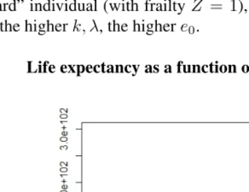
keeping all other parameters fixed, which is intuitively justified asadenotes the starting level of mortality. A little counterintutive is the finding that life expectancy increases as the rate of agingb=dlnµ(x)/dxincreases (see Figure 1). The gamma parameterskand λ, often assumed to be equal to one another, so thatµ(x)denotes the force of mortality of the “standard” individual (with frailtyZ = 1), have one and the same impact on life expectancy – the higherk, λ, the highere0.
Figure 1: Life expectancy as a function ofb.
Notes: Life expectancy at birth as a function ofbfor fixeda= 5×10⁻⁷,k=λ= 7.
Note that when baseline mortalityµ(x)in (1) is Gompertz-Makeham, i.e.
µ(x) =aebx+c ,
Demographic Research: Volume 28, Article 9
µ(x|Z) =Z(aebx+c),
the corresponding life-expectancy integral
e0= ∞
Z
0
1− a
bλ+ c λx+
a bλe
bx−kdx
cannot be solved analytically, even for integer values ofk.
As already pointed out, for human populations we have1−a/bλ≈1, which leads to further simplification of (4):
(7) e0≈
1 b lnbλ a − k−1 X j=1 1 j
Note that whenk=λ(often assumed, see Vaupel, Manton, and Stallard (1979)), the right-hand side of (7) contains the difference between the partial sum of the harmonic series and the natural logarithm:
(8) e0≈
1 b ln b a+ 1 k− k X j=1 1
j −lnk
.
The limit of the latter when k → ∞ is the Euler-Mascheroni constant γ∗ ≈ 0.577. Note that k → ∞ corresponds to the case when the Gompertz model for a gamma-heterogeneous population tends to the Gompertz model for a homogeneous population. As a result, life expectancy at birth for a homogeneous population experiencing a Gom-pertz force of mortality could be approximated by
(9) e0≈
1
b
lnb
a−γ
∗
.
I:=
Z
1 + a
bλ e
bx−1−k
dx=
Z bλ
ae
−bx
k
1−
1−bλ
a
e−bx
−k
dx .
Ay=e−bxsubstitution will result in
I=−1 b
bλ
a
kZ
yk−1
1−
1−bλ
a
y
−k
dy .
Taking into account (see Lebedev 1965, p.258)
1−
1−bλ
a
y
−k = 2F1
k, C;C;
1−bλ a
y
∀C≡const
and2F1(α, β;γ;z) = 2F1(β, α;γ;z),we have
1−
1−bλ
a
y
−k = 2F1
k, k;k;
1−bλ a
y
.
Using in addition (see MathWorld 2012, http://functions.wolfram.com/07.23.21.0006.01)
Z
zγ−12F1(α, β;γ;z)dz=
zγ
γ 2F1(α, β;γ+ 1;z) and switching back to the original variablex, we reduce (6) to
I=−1 bk bλ ae −bx k
2F1
k, k;k+ 1;
1−bλ a
e−bx
.
Taking into account
lim x→∞ ( −1 bk bλ a e −bx k
2F1
k, k;k+ 1;
1−bλ a
e−bx
)
= 0,
we finally get
(10) ex= 1
bk
bλ
ae
−bx
k
2F1
k, k;k+ 1;
1−bλ a
e−bx
Demographic Research: Volume 28, Article 9
4.
Applications
Relationship (2) and its approximation (4) can be used to measure the difference between actual (calculated by lifetable methods) and model-predicted (based on the estimation of gamma-Gompertz parameters) life expectancy at birth. This difference quantifies the cumulative excess infant and adult mortality. Figure 2 illustrates this gap for Swedish females from 1891 to 2010. As infant mortality improves over time, the difference de-creases from 1950 onwards to an almost constant value of about 2 years.
If we use expression (10) or its approximation (for integerk) analogous to (4), we can see that the gap between actual and fitted gamma-Gompertz remaining life expectancy decreases over agex(see Figure 3). This illustrates on aggregate the phenomenon that most deaths which are not captured by the gamma-Gompertz model, occur from infant to young adult ages.
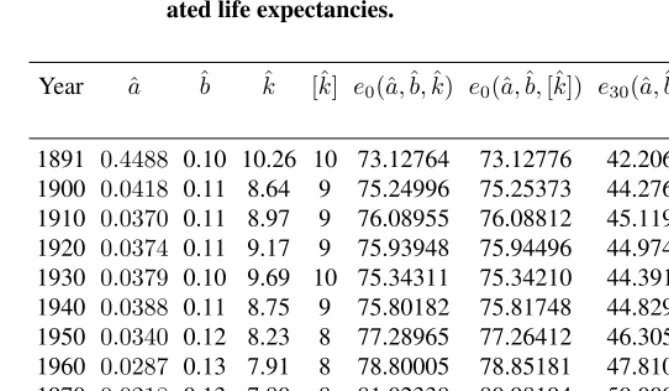
Empirically, it does not make a significant difference whether life expectancy is calcu-lated in terms of the hypergeometric function (2) or by approximation (4). I use the data for Swedish females (HMD 2012) to estimate parametersa,b, andk(assumingk=λ) by miximizing a Poisson likelihood of the respective death counts. I start at age70, assuming the baseline force of mortality onwards to be purely Gompertz, and calculate the initial mortality level by multiplying the estimatedˆabyexp{(initial age−70)ˆb}, whereˆbis the maximum-likelihood estimate ofb. Table 1 shows observed and fitted gamma-Gompertz life expectancies at birth and at age30for Swedish females in several specified years, il-lustrating how close these values are, regardless of the proximity ofkˆto its closest integer
[ˆk]. This implies that one can use (4) instead of (2) without losing much precision. Approximations (7) and (8) are not very accurate as small deviations a/bk(k = λ) from1can lead to substantial deviations from (4) and, thus, from (2). They can be used, though, to assess the impact of model parameters on the values of life expectancy at birth.
5.
Conclusion
Life expectancy in a gamma-Gompertz multiplicative model can be expressed analytically in terms of a special function (the hypergeometric series), which provides insight on life expectancy dynamics with respect to model parameters. In practice, one can use high-accuracy approximation (4) instead of (2) to calculate model-basede0for fitted parameter
Figure 2: Actual vs gamma-Gompertz life expectancy at birth.
Notes: Actual vs gamma-Gompertz life expectancy (Data source: HMD (2012), Sweden, females; own estimation).
Figure 3: Actual vs gamma-Gompertz life expectancy.
Demographic Research: Volume 28, Article 9
Table 1: Maximum-likelihood estimates for model parameters and associ-ated life expectancies.
Year ˆa ˆb ˆk [ˆk] e0(ˆa,ˆb,kˆ) e0(ˆa,ˆb,[ˆk]) e30(ˆa,ˆb,kˆ) e30(ˆa,ˆb,[ˆk])
1891 0.4488 0.10 10.26 10 73.12764 73.12776 42.20659 42.20671 1900 0.0418 0.11 8.64 9 75.24996 75.25373 44.27699 44.28077 1910 0.0370 0.11 8.97 9 76.08955 76.08812 45.11981 45.11837 1920 0.0374 0.11 9.17 9 75.93948 75.94496 44.97437 44.97984 1930 0.0379 0.10 9.69 10 75.34311 75.34210 44.39173 44.39073 1940 0.0388 0.11 8.75 9 75.80182 75.81748 44.82903 44.84469 1950 0.0340 0.12 8.23 8 77.28965 77.26412 46.30584 46.28031 1960 0.0287 0.13 7.91 8 78.80005 78.85181 47.81052 47.86228 1970 0.0218 0.13 7.80 8 81.02338 80.98194 50.00065 49.99920 1980 0.0180 0.13 7.66 8 82.37141 82.40531 51.39669 51.40060 1990 0.0147 0.13 7.62 8 83.70550 83.70612 52.71329 52.70737 2000 0.0119 0.14 7.40 7 85.10804 85.12865 54.10920 54.11260 2010 0.0091 0.14 7.12 7 86.53489 86.53414 55.49925 55.49785
Notes: Maximum-likelihood estimatesaˆ(at age 70),ˆb,ˆkof the gamma-Gompertz parameters and respective life expectancies:e0(ˆa,ˆb,ˆk)calculated by (2),e0(ˆa,ˆb,[ˆk])calculated by (4),e30(ˆa,ˆb,ˆk)calculated by (10),
ande30(ˆa,ˆb,[ˆk])calculated by a formula analogous to (4) (Data source: HMD (2012), Sweden, females;
own estimation).
6.
Acknowledgements
References
Abramowitz, M. and Stegun, I. (1965).Handbook of Mathematical Functions. Washing-ton, DC: US Government Printing Office.
Bailey, W.N. (1935).Generalised Hypergeometric Series. Cambridge: University Press.
Beard, R.E. (1959). Note on some mathematical mortality models. In: Woolstenholme, G. and O’Connor, M. (eds.).The Lifespan of Animals. Little, Brown and Company: 302–311.
Finkelstein, M.S. and Esaulova, V. (2006). Asymptotic behavior of a general class of mixture failure rates. Advances in Applied Probability 38(1): 244–262.
doi:10.1239/aap/1143936149.
HMD (2012). The human mortality database. [electronic resource]. URL: http://www.mortality.org.
Keyfitz, N. and Caswell, H. (2005). Applied Mathematical Demography. New York: Springer, 3rd ed.
Lebedev, N.N. (1965).Special Functions and Their Applications. Englewood Cliffs, N.J.: Prentice-Hall.
MathWorld (2012). Wolfram mathworld. [electronic resource]. URL: http://mathworld.wolfram.org.
Vaupel, J.W. (2008). Supercentenarians and the theory of heterogeneity. [unpublished manuscript]. Rostock: Max Planck Institute for Demographic Research. Johann Süßmilch Lecture Series in 2008/2009.
Vaupel, J.W., Manton, K.G., and Stallard, E. (1979). The impact of heterogeneity in individual frailty on the dynamics of mortality. Demography 16(3): 439–454.