Economic Analysis of Price Shocks of Production Inputs and
Their Impact on Cotton Price in Iran: The Application of Panel
Data Vector Auto-Regression (PVAR) Model
Ali Sardar Shahraki*, Neda Ali Ahmadi, Mahdi Safdari
University of Sistan and Baluchestan, Zahedan, Iran
Received: 15 July 2018 /Accepted: 11 December 2018
Abstract
Cotton is a strategic crop with a critical role in the economy and agriculture. The increasing price of crop inputs is the main challenge for the developing countries, including Iran, so that it is crucial for the economy of the states to recognize the underpinning factors. Accordingly, the present study aimed to identify the relationship between price shocks of cotton production inputs and cotton price in 12 provinces of Iran over the 2000-2016 time period using panel-data vector auto regression (PVAR) model. The results to estimate the model and to check the interrelationships of the research variables in the context of the impulse response functions and analysis of variance showed that the variables of seed price, labor price, and pesticide price have a significant positive relationship with cotton price with the numerical values of 0.296, 0.002 and 0.017, respectively. The relationship of the variables of land and fertilizer prices was found to be negative but non-significant with the numerical values of 8.23 and 0.118, respectively. According to the results, to avoid the price volatility and shocks in input and output markets, it is recommended to organize and regulate the demand and supply system of the inputs and output.
Keywords: Economic Analysis, Price Shock, Agricultural Input, Cotton, Panel Vector Autoregression
Introduction
Cotton, the white gold, is one of the most valuable industrial crops and is a key product of the agricultural sector with an essential role in this sector and the industrial sector (Ghasemian et al., 2014). Statistics show that cotton accounts for 75 percent of the total natural fiber production in the world. Cottonseed is the second most important oilseed in the world (Haeri & Asayesh, 2009; Fathi et al., 2011). Also, this crop plays a vital role in the supply of raw material for textile industry, oil production, and employment in the agricultural, industrial and commercial sectors (Rostami et al., 2017). According to the crop statistics of 2015-2016, Iran annually produces 161,164 t cotton. The total harvesting area of this crop in Iran is estimated at about
14.4 million ha. Irrigated farms produce 159,075 t cotton and rain-fed farms produce 2,088 t. The yield of the irrigated farms is 2,302 kg ha-1, while rain-fed farms report a yield of 1,371
kg ha-1. Also, the acreage of irrigated cotton is 69,102 ha and that of rain-fed cotton is 1,523 ha
(Crop Statistic Book, 2016).
One of the most basic foundations of neoclassical economics is the theory of price. Prices are among the main determinants of the income level of farmers, importers and exporters of the agricultural products as well as the economic welfare of consumers (Hosseini & Nikoukar, 2006; Frigon et al., 1999; Campenhout et al., 2018; Charley & Rohan, 2018). The analysis of crop prices is important from the economic and political perspectives. So, most agricultural economists have focused on the structure of the relevant markets (from farm to retail) and the process of price transmission (Hosseini & Dourandish2006; Broson et al., 1985; Wharton, 2017; Hussein, 2018). A major issue faced by people and policymakers at the macro level is the price volatility of the agricultural commodities because these volatilities are a barrier against the improvement of the productivity of the agricultural sector. These volatilities are blamed for the increase in inflation pressures. Inflation by itself makes agricultural production a risky activity, and this affects investment decisions, thereby having dramatic consequences for farmers, growth, income, productivity, and profitability (Kargbo, 2005; Wang et al., 2017; Joets et al., 2017; Alan Ker et al., 2017; Seth & Sidhu, 2018; Url et al., 2018). In this regard, crop price is mainly influenced by the price of the inputs and their relationship with the crop price in the agricultural sector, and this has been considered by many researchers. Therefore, to analyze agricultural crop markets, it is imperative to understand the relationship between input and crop and their pricing effect on one another in order to use it for the sake of sound policymaking (Marab & Moghadasi, 2007; Bailey Norwood & Lusk, 2018; Alizadeh & Handifield, 2018).
Given the significance of the research, an essential feature of the agricultural crops is the volatility of their prices at different market levels. Since most studies in Iran have focused on the transmission of price from producers to retailers on the one hand and cotton is a key crop with high economic value due to its extensive applications on the other hand, it is imperative to assess the effects of price shocks of cotton inputs (labor, seed, land, pesticide, fertilizer, and water) on the price of cotton in Iran. So, the present study aims to use vector auto-regression model with panel data (PVAR) to answer the question as to how price shocks of cotton production inputs affect its production and price.
Literature Review
prices on the prices of the agricultural crops.
From the perspective of statistical methodology, the study of the relationship between variables has evolved through four phases. The first phase was based on vector auto-regression method (VAR) in that the property of the stationarity of the variables was neglected. In the second phase, given the non-stationarity of the variables, the two-stage process of Engle-Granger was used to test the cointegration relations of two variables. In the third phase, multivariate predictors like Johansen were applied in which more than two variables were applicable in cointegration relations and causality analysis. In the fourth phase, the research was based on unit root test, cointegration test and causality test of Granger or others (Shahateet, 2014; Tarfirenyika, 2017; Amin & Alam, 2018; Molele & Ncanywa, 2018). Given the many advantages of panel data methods, panel data-based vector auto-regression model (PVAR) can be used to cope with the statistical limitations and uncertainty about the exogeneity of the variables in time-series model in short periods. PVAR encompasses the conventional VAR method, and the only difference is that it uses panel data (Jafari Samimi et al., 2009; Amoli Diva & Jafari Samimi, 2010; Jouida, 2018; Thach & Oanh, 2018). The PVAR approach is a non-structural approach that is employed to model the relations among multiple variables (Love and Ziccino, 2006). PVAR works with the same rationale of VAR. What is important in VAR models is to apply the shocks and to trace their results. In PVAR models, shocks can be recognized with standard methods (Mohammadzadeh Asl, 2017). In this regard, the following research can be noted.
Farajzadeh and Ismaili (2010) studied price transmission in pistachio markets in two parts – time series (1972-2005) and panel data (1989-2005). They found a long-run reciprocal relationship between domestic price and global price of pistachio. The results of time series analysis revealed a long-run symmetric pattern of transmission in both the domestic and global markets of pistachio. Also, the results of hybrid data showed that the multiplicity of the countries importing Iran’s pistachio had a decreasing trend and that the increase in their share in purchase market and the decrease in Iran’s share of the global market has resulted in symmetric price transmission between the domestic and global markets. Mohammadi et al. (2015) used the sensitivity analysis in artificial neural network model to conduct an empirical study on the trend of exchange rate pass-through and the effect of its volatility on pistachio export price in Iran in 1961-2011. The results showed a direct relationship between exchange rate fluctuations and pistachio export price. So, in case of the decline of exchange rate volatility, exporting pistachio can be supplied at lower prices to the global markets, and given the elasticity of the global demand, the incomes of exporting this crop are enhanced.
price fluctuations and shocks in input market can contribute to stabilizing maize crop price. Also, Parsley (2012) worked on the extent of exchange rate pass-through in South Africa using panel data over the 1998-2009 period. They found that the pass-through of exchange rate variations to import price was 60 percent. Zare Mehrjerdi and Tohidi (2014) applied dynamic panel data model and GMM to study exchange rate and tariff pass-through to saffron export price in 2000-2011. They found that the exchange rate pass-through to saffron export price was incomplete. Da Silveira and Mattos (2015) focused on the transmission of price and volatility between feed and livestock markets in the US and Brazil during 1996-2014 using vector error correction method. According to their findings, price volatilities has changed between feed markets in the US in the short and long run, but the volatilities in Brazil just existed in the short run. Mekbib et al. (2016) examined the effect of price volatility of the products and inputs on wheat, rice, maize, and soybean using the panel data approach. The results showed that supply price elasticity varied in the range of 0.04-0.05. On the other hand, price volatility was negatively related to supply. Ojewumi and Akinlo (2017) considered foreign direct investment, economic growth and environmental quality in sub-Saharan Africa using a dynamic model. They reported dynamic interactions among foreign direct investment, economic growth and environmental quality whereas their effect on one another varied in the range of 13.1-32.8 percent. As well, the member states of Southern Africa should make a balance between investment policies and environmental conservation policies so that foreign direct investment is increased in the region, resulting in the improvement of the environmental quality of the local countries. A review of the empirical studies shows that they have mostly focused on price transmission and no study has assessed the price shock transmission from inputs market to commodity market. On the other hand, most models have used time series data, while models have not utilized hybrid data, which are of high analytical power. The application of simultaneous equations system and the examination of the long-term relationship between market variables via PVAR, the assessment of the impacts of instantaneous shocks of each individual market variable on cotton price in the context of impulse response function (IRF) and the determination of the long-term relations of these variables (the price of the production factors and output) are issues that should be assessed due to the significance of agriculture and its products in new studies in agriculture economics. Therefore, the present study aims to use panel vector autoregression (PVAR) model to analyze the price in input and output market and their price shocks.
Materials and methods
variables. Second, it has been designed to show the problem of endogeneity (Lin and Zhu, 2017). As such, VAR models alleviate the problem of endogeneity without applying unnecessary constraints. Third, VAR-based IRFs can consider the lagging impacts on variables and the effect of shocks whilst these dynamic impacts are not shown by PVAR models. Fourth, PVAR models allow considering the fixed cross-provincial (cross-sectional) and cross-time impacts. Finally, PVAR can also be used in relatively short time-series using cross-sectional dimension (Grossmanna et al., 2014; Galariotis et al., 2018). PVAR is structurally expressed as:
(1)
So that the sequences y1it and y2it are stationary. ε1it and ε2it are error terms with the variances
ω1 and ω2, respectively. They are independent of one another. The maximum number of lags
included in these equations is one lag. So, these equations form the structural form of the first-order PVAR. The structure of the system is so that it allows either variable to influence the other. However, if b12 ≠ 0, ε1it will have an indirect impact on y2it, and if b22≠ 0, ε2it will have
an indirect impact on y1it. The simultaneous effectiveness of y1it and y2it, as well as y2it and y1it,
reflects the fact that these equations do not have a reduced form. If the above structural form is rewritten in the matrix form, the equations will be changed to (Hayakawa, 2016):
(2)
Equation (2) is for the bivariate state. The structural form of PVAR for the n-variate state is as below:
(3)
Despite the feedback mechanism†, Equations (1) and (2) cannot be estimated in the structural
form. To solve this problem, one needs the solved form of PVAR. The structure form is transformed into the solved form by the following equation (Hayakawa, 2017):
(4)
The solved form can be written in more complete form as below:
† The correlation of y2it with error term ε1it and the correlation of y1it with ε2it create the feedback mechanism.
12 10 11 12 1
1 2 1 , 1 2 , 1
21 1 2 20 21 1 , 1 22 2 , 1 2
y it b y it y i t y i t it
y y y y
b it it i t i t it
g g g e
g g g e
+ = + - + - +
+ = + - + - +
1 (0, )
2 it N it e e æ ö » W ç ÷ ç ÷
è ø where
2 0 1 2 0 2 w w æ ö ç ÷
W=ç ÷
ç ÷ è ø ) , 0 ( , 1 1 1 , 1 0 2 1 1 , 2 1 , 1 22 21 12 11 20 10 2 1 21 12 W » e e + G + G = Þ ú û ù ê ë é e e + ú û ù ê ë é ú û ù ê ë é g g g g + ú û ù ê ë é g g = ú û ù ê ë é ú û ù ê ë é -N y By y y y y b b it it t i it it it t i t i it it
1 , 1 ....
1 10 11 12 13 1
.... 2 , 1
2 20 21 22 23 2
.
3 30 3 , 1
. . . . . . . . . . . . ....
0 1 2 3 , 1
Y i t
Y it Y n
Y i t
Y it Y n
Y it Y Y i t
Ynit Yn n n n nn Y ni t
g g g g
g g g g
g g g g
é ù é ù -é ù é ù ê ú ê ú ê ú ê ú ê -ê ú ê ú ê ú ê ê ú ê ú ê ú ê -ê ú ê ú ê ú ê = +ê ú ê ú ê ú ê ê ú ê ú ê ú ê ê ú ê ú ê ú ê ê ú ê ú ê ú ê ê ú ê ú ê ú ê ë û ë û ë ûë - û 1 2 3 . . . it it it nit e e e e é ù ê ú ú ê ú ú ê ú ú ê ú ú+ê ú ú ê ú ú ê ú ú ê ú ú ê ú ú ë û
12 12 12
10 20 11 21 12 22 1 12 2
1 1 1 1 , 1 1
1 21 12 21 12 21 12 21 12
21 10 20 21 11 21 21 12 22
2 2 , 1
1 1
1 21 12 21 12 21 12
b b b it b it
y
y it b b b b b b i t b b
y it b b b y i t
b b b b
b b
g g g g g g e e
g g g g g g
é - ù é - - ù -ê ú ê ú é ù é ù ê - ú ê - - ú ê - -ú ê ú=ê ú ê+ ú ê + ú + + + - - -ê ú -ë û ê ú ê úë û - -ê ú êë úû ë û
21 1 2 1 21 12
b it it
(5)
(6)
Model (6) is a standard PVAR model. Equation (5) is estimated by ordinary least squares (OLS) method. But, we can derive data for the structural form from the results of estimating the summarized form. This is due to the fact that by estimating the second system, it is possible to estimate the variables α22, α21, α12, α11, α20, α10, σ12, σ22, and σ12 if the initial equations system
have 10 parameters including γ20, γ10, γ22, γ21, γ12, γ11, b21, and b12 and two standard deviations
of ω12 and ω22. In other words, the structural form has 10 parameters, and in the solved form of
the PVAR model, 9 parameters are estimated. Therefore, it is not possible to identify the initial equations system without considering constraint on one of the parameters (Sharifi Renani et al., 2013). On the other hand, if in the PVAR structural form, it is assumed that the coefficient b12
or b21 is zero, the structure form will be as below (in which it is assumed that b21 = 0)‡:
In this state, y2it has a simultaneous effect on y1it, but y1it affects y2i with one lag. The application
of the constraint that one of the coefficients b12 or b21 be zero enables us to base the model on
the theory of economy. Also, this condition tackles the problem of identifying and restoring the coefficients of the structural form from the results of the solved form estimation (Asid et al., 2012; Juodis, 2017).
According to the explanations, the present study used the following VAR model:
The model was estimated by data for the cotton crop of 12 provinces in Iran for the time period of 2000-2016 using the Eviews 10 software package. The variables included cotton crop
‡ This is extracted from recursive method presented by Simens (1980) for identifying VAR equations, which can
be generalized to the PVAR model.
1 , 1
1 10 11 12 1
20 21 22 2
2 2 , 1
y
y it i t eit
y it y i t e it
a a a
a a a
é ù é ù é ù é ùê - ú é ù ê ú=ê ú+ê ú +ê ú ê ú ê ú ë û ë û - ë û ë û ë û
1 (0, ) 2
e it N
e it æ ö
» S
ç ÷ ç ÷
è ø where
2 12 1 2 12 2 s s s s é ù ê ú
S =ê ú
ê ú
ë û
0 1 , 1
yit A A Ai t eit
Þ = + - + eit »N(0, )S
where A0=B-1 ,G0 A1=B-1G1 and eit =B-1eit
12 10 11 12 1
1 2 1 , 1 2 , 1
2
20 21 22
2 1 , 1 2 , 1
y it b y it y i t y i t it
y it y i t y i t it
g g g e
g g g e
+ = + - + - +
= + - + - +
11
10 1 12 1 13 1 14 1 15 1 16 1 17 1 1
21
20 1 22 1 23 1 24 1 25 1 26 1 27 1 2
31
30 1 32 1 3
b py
pyit b b it pbit b plit b plait b psit b pshit b pwit it
b py
pbit b b it pbit b plit b plait b psit b pshit b pwit it
b py
plit b b it pbit
e e + = - - - + - + - + - + - + - + + = - - - + - + - + - + - + - + +
= - - - + 3 1 34 1 35 1 36 1 37 1 3
41
40 1 42 1 43 1 44 1 45 1 46 1 47 1 4
51
50 1 52 1 53 1 54 1 55 1
pl pla ps psh pw
b it b it b it b it b it it
b py
plait b b it pbit b plit b plait b psit b pshit b pwit it
b py
psit b b it pbit b plit b plait b psit
e e + + + + + - - - - -+ = - - - + - + - + - + - + - + +
= - - - + - + - + - 56 1 57 1 5
61
60 1 62 1 63 1 64 1 65 1 66 1 67 1 6
71
70 1 72 1 73 1 74 1 75 1 76 1 77 1 7
psh pw
b it b it it
b py
pshit b b it pbit b plit b plait b psit b pshit b pwit it
b py
pwit b b it pbit b plit b plait b psit b pshit b pwit it
price (PY), labor price (PL), seed price (PB), land lease price (PLA), pesticide price (PS), fertilizer price (PSH), and water price (PW) derived from the statistic book of Jihad-e Agriculture Ministry. All data are yearly in logarithmic form.
Empirical Results
Unit root tests of panel data
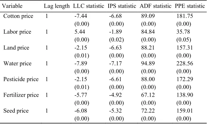
Before model estimation, we need to test the stationarity of all variables used in model estimation because the stationarity of the variables is a source of spurious regression for both time series and panel data types. Unit root expresses that unit root test based on panel data is more robust and correct that the test based on time series data (Salimi Far and Dehnavi, 2009; Jouida, 2018; Thach and Oanh, 2018). We employed the tests of Levin, Lin, and Chu (LLC), Im, Pesaran and Shin (IPS), augmented Dickey-Fuller (ADF), and Phillips and Perron (PPE) for unit root test of the panel data. The results are summarized in Table 1, according to which all variables were made stationary by first-differencing.
Table 1. Results of panel unit root tests for cotton crop
Variable Lag length LLC statistic IPS statistic ADF statistic PPE statistic Cotton price 1 -7.44 -6.68 89.09 181.75
(0.00) (0.00) (0.00) (0.00)
Labor price 1 5.44 -1.89 84.84 35.78
(0.00) (0.02) (0.00) (0.05)
Land price 1 -2.15 -6.63 88.21 157.31
(0.01) (0.00) (0.00) (0.00) Water price 1 -7.89 -7.17 94.89 228.56
(0.00) (0.00) (0.00) (0.00) Pesticide price 1 -2.15 -6.61 88.00 172.29
(0.01) (0.00) (0.00) (0.00) Fertilizer price 1 -5.77 -4.92 67.12 138.90
(0.00) (0.00) (0.00) (0.00)
Seed price 1 -6.08 -5.32 72.22 159.01
(0.00) (0.00) (0.00) (0.00)
Since the variables were made stationary by first-differencing, panel cointegration test was applied to ensure the feasibility of including the variables in the model because in panel data, if there exists a cointegration among the variables, it is not necessary to make the data stationary, and if stationarity test is refuted for the variables, it is necessary to perform cointegration test. Thus, in case the variables are cointegrated, the results will be reliable (Nasir and Du, 2018). There are some tests including the Kao, Pedroni, and Fisher tests to examine cointegration. We employed the Kao test to prove that regression was not spurious. The Pedroni test could not be used due to the high number of model variables, and the Fisher test could not be applied due to the inadequacy of data (Gamtessa and Olani, 2018).
Table 2. Results of panel cointegration test using the Kao test for cotton crop
Kao cointegration t-statistic Probability
ADF -6.27 0.00
PVAR model estimation
Determining optimal lag length
The selection of an optimal lag length is a very important step in PVAR models so that correct forecasts depend on this selection. Small lags may be unable to reflect the dynamic of the system and cause the problem of the variable elimination from the model. They may also make the residual of the coefficients biased, which is likely to create correlated errors. On the other hand, very large lags may erode degrees of freedom rapidly and lead to over parameterization (Abrigow and Low, 2015). To find out the optimal lag in an econometric model, all variables are estimated in the context of a VAR equation using such statistics as the Akaike information criterion (AIC; Akaike, 1969), the Bayesian information criterion (BIC; Schwartz; Akaike, 1977), and the Hannan-Quinn information criterion (HQIC; Hannan and Quin, 1979) which is calculated by the logarithm of the likelihood function. The lag that has the lowest Akaike, Schwartz, and Hannan-Quinn values constitutes the optimal lag number (Noferesti, 2008). Table 3 presents the results of tests for determining optimal lag of the model.
Table 3. Results of the test to determine optimal lag for VAR
Lag Log L LR FPE AIC SC HQ
0 -7123.167 NA 5.21e+48 132.0401 132.2140 132.1106
1 -6651.474 873.5058* 2.08e+45* 124.2125* 125.6032* 124.7764* 2 -6614.539 63.60972 2.63e+45 124.4359 127.0435 125.4923 3 -6596.255 29.11871 4.78e+45 125.0047 128.8293 126.5554 4 -6575.604 30.21286 8.52e+45 125.5297 130.5711 127.5738 5 -6545.497 40.14282 1.32e+46 125.8796 132.1379 128.4171 6 -6516.362 35.06871 2.20e+46 125.2475 133.7227 129.2784 7 -6498.220 19.48603 4.80e+46 126.8189 135.5110 130.3432 8 -6443.803 51.39392 5.84e+46 126.7186 136.6276 130.7363
According to Table 3, all three criteria of Akaike, Schwartz, and Hannan-Quinn determined the lag number of 1 as the optimal lag for cotton crop in Iran.
Model estimation
Table 4 shows the results of the model estimation to test cotton price relationship with the price of inputs including labor, seed, land (land lease), fertilizer, pesticide, and water.
Table 4. Results of model estimation by vector auto-regression method for cotton crop
PB PL PLA PS PSH PW PY
PW(-1) 0.524 -0.795 27.878 0.211 0.001 -52.314 0.296 (0.078) (0.520) (30.153) (0.797) (0.019) (30.010) (0.141) [6.714]** [-1.528]* [0.924] [0.264] [0.075] [-1.743]** [2.097]**
PL (-1) 0.015 0.986 -0.168 0.072 0.001 3.630 0.002
(0.004) (0.029) (1.726) (0.045) (0.001) (1.718) (0.008) [3.375]*** [33.116]*** [-0.097] [1.583]* [1.514]* [2.112]** [0.253]** PLA (-1) 2.51 0.0008 0.916 -0.0008 -3.15 -0.087 -8.23
(0.00) (0.0006) (0.039) (0.001) (2.6) (0.039) (0.0001) [0.243] [1.256] [23.049]*** [-0.846] [-1.22] [-2.203]** [-0.440]
PS (-1) 0.011 -0.038 1.169 0.793 0.001 2.735 0.017
(0.005) (0.033) (1.934) (0.051) (0.001) (1.925) (0.009) [2.240]*** [-1.153] [0.604] [15.50]*** [0.986] [1.420]* [1.893]** PSH (-1) 0.348 2.444 11.574 -1.387 0.783 -4.941 -0.118
(0.254) (1.696) (98.359) (2.602) (0.063) (97.894) (0.461) [1.367]* [1.440]* [0.117] [-0.533] [12.284]*** [-0.050] [-0.256] PW (-1) -0.0003 -0.0004 -0.087 0.001 2.43 0.852 0.0002
(0.0001) (0.001) (0.061) (0.001) (4.0) (0.060) (0.0002) [-2.287]** [-0.467] [-1.431]* [0.976] [0.612] [14.011]*** [1.030] PY (-1) 0.148 -0.095 -15.762 0.028 0.019 25.799 0.738
(0.045) (0.303) (17.571) (0.464) (0.011) (17.488) (0.082) [3.264]*** [-0.467] [-0.897] [0.062] [1.703]** [1.475]* [8.957]***
After the PVAR model is estimated, the next important step is to check the interrelationships and the dynamic relationships of the model variables. According to the subject matter, this section deals with the impact of the price of labor, seed, pesticide, fertilizer, land, and water on cotton price.Figure 1 depicts the dynamic response of the variable of cotton price to the shocks in the descriptive variables. In these graphs, the x-axis is time and the y-axis is the deviation from the initial value. Also, the lines drawn in the middle represent the impulse responses of the cotton price up to 10 periods. The upper and lower lines are the positive and negative bounds for the standard deviation of the impulse responses at the p < 0.05 level, which has been calculated with 1000 repetitions using the Monte Carlo simulation.
Figure 1. The dynamic response of cotton price to shocks to the descriptive variables of the model
After examining IRFs, we turn to the analysis of variance (ANOVA) for cotton crop. Whilst IRFs reflect the response of an endogenous variable over time to a shock induced by another variable of the system, ANOVA measures the contribution of each shock to the variance of an endogenous variable of the system. The results of ANOVA for the cotton crop are summarized in Table 5.
Table 5. Analysis of variance for cotton price
Period PB PL PLA PS PSH PW PY
1 22.976 0.505 0.003 1.348 14.705 7.246 53.214
2 30.170 0.389 0.046 0.784 13.563 7.760 47.285
3 34.275 0.290 0.172 1.025 12.910 8.017 43.309
4 36.397 0.308 0.370 1.735 12.547 8.181 40.460
5 37.292 0.866 0.909 3.556 12.278 8.467 36.495
7 37.083 1.422 1.217 4.378 12.276 8.625 34.995
8 36.445 2.151 1.532 5.053 12.329 8.798 33.689
9 35.628 3.033 1.843 5.563 12.420 8.982 32.528
10 34.710 4.047 2.140 5.914 12.538 9.170 31.477
Since the forecast error of each year is estimated on the basis of the previous year error, so the forecast errors have a descending trend over the studied period. The columns in Table 5 show the percentage of the forecast variance due to different shocks in which the sum of each
-3 -2 -1 0 1 2 3 4
1 2 3 4 5 6 7 8 9 10 Response of PY to PY
-3 -2 -1 0 1 2 3 4
1 2 3 4 5 6 7 8 9 10 Response of PY to PB
-3 -2 -1 0 1 2 3 4
1 2 3 4 5 6 7 8 9 10 Response of PY to PL
-3 -2 -1 0 1 2 3 4
1 2 3 4 5 6 7 8 9 10 Response of PY to PLA
-3 -2 -1 0 1 2 3 4
1 2 3 4 5 6 7 8 9 10 Response of PY to PS
-3 -2 -1 0 1 2 3 4
1 2 3 4 5 6 7 8 9 10 Response of PY to PSH
-3 -2 -1 0 1 2 3 4
1 2 3 4 5 6 7 8 9 10 Response of PY to PW
row is 100 percent.
According to the results, in the 1st period, 53.2 percent of the cotton price variance is accounted for by the variable itself and the remaining is captured by other variables. In the 2nd period, 47.2 percent of the cotton price variance is explained by cotton price, 30.1 percent by seed price, and the remaining by other variables. In the 3rd period, cotton price accounts for 43.3 percent of the cotton price variance, seed price accounts for 34.2 percent, and the remaining is captured by the forecast error of other variables. In the 4th to 10th periods, cotton price accounts for 40.4, 38.2, 36.4, 34.9, 33.6, 32.5, and 31.4 percent of the cotton price variance, respectively; seed price accounts for 36.3, 37.2, 37.4, 37.0, 36.4, 35.6, and 34.7 percent of its variance, respectively; and the remaining is related to the other variables. In other words, it can be observed that over time, the role of cotton price diminishes drastically and seed price gains higher and higher importance so that in the 10th period, 34.7 percent of the variance is captured by the seed price.
Conclusions and Recommendations
With respect to the significance of cotton price in Iran, this study addressed the question as to how much cotton price volatility is influenced by the price shocks of cotton production inputs including labor, land, seed, pesticide, fertilizer, and water. After the optimal lag was specified and the long-run relationship between the variables was determined, the cointegration relationships were employed to find out the variables influencing cotton price volatility in Iran over the time period of 2000-2016 using the PVAR method. The results showed that the price shocks of seed, labor, pesticide, and water have affected cotton price positively, and the variations between seed price increase and the variations of cotton price growth have been of crucial importance. Thus, at purchase time, this should be considered because the increase or decrease in seed price is a decisive factor in cotton pricing in the marketplace. The effect of water price was found to be insignificant because water is supplied to farmers in most regions free of charge or at very low prices. So, it has a very minor role among decisive factors. The variables of land and fertilizer price shocks have influenced cotton price negatively. In case of land, this can be explained by the fact that most farmers are the owners of their lands, so land lease cost does not emerge among implicit costs, leading to its negative impact on cotton price. The negative impact of fertilizer price shock on cotton price is induced by the variations of other factors. The price of pesticide cannot be explained and the results showed that it has not influenced cotton price considerably. This research is consistent with the results of studies by Moradi and Afsharmanesh (2017) and Mekbib et al. (2016).
can be attained in the marketplace and the producers are directed towards a suitable atmosphere to sell their products. Supporting this union can contribute to solving some problems faced by the producers.
References
Akaike, H. (1969). Fitting autoregressive models for prediction. Annals of the institute of Statistical Mathematics, 21: 243-247.
Alan Ker, N. L; Sam, A and Aradhyula, S. (2017). Modeling regime-dependent agricultural commodity price volatilities. Agricultural economics, 48(6): 683-691.
Alizadeh, H.M and Handifield, R. (2018). IEEE Transactions on Engineering Management, 99:1-14. Amin, S. B and Alam, T. (2018). The Relationship Between Energy Consumption and Sectoral Output
in Bangladesh: An Empirical Analysis, The Journal of Developing Areas, 52(3): 39-54.
Amoli Diva, K., and Jafari Samimi, A. (2010). The effect of fiscal freedom on government efficiency in terms of economic liberalization (The case of OIC countries. Tax Research, 18 (8), 81-102. (In Persian)
Asid, R. Kogid, M. Mulok, D and Lily, J. (2012). Intellectual Property Rights Protection, Foreign Direct Investment and Economic Growth in Malaysia: An ARDL Bound Test Approach. Asian Journal of Empirical Research ,2(2): 9-19.
Bailey Norwood, F and Lusk, J. (2018). Agricultural Marketing and Price Analysis. Technology & Engineering, Page, 445.
Brorson, B.W., Chavas, J.P., Grant, W.R., Schanke, L.D. (1985). Marketing margins and price uncertainty: The Case of the U.S. Wheat Market. Amer. J. Agr. Econ., 67: 521-28.
Campenhout, B. V, Pauw, K and Minot, N. (2018). The impact of food price shocks in Uganda: first-order effects versus general-equilibrium consequences, European Review of Agricultural Economics, https://doi.org/10.1093/erae/jby013.
Charley, X and Rohan, N. (2018). Exploring Australia's comparative advantage for exporting fresh produce, Agricultural Commodities, 8(1): 176-198.
Crop Statistic Book (2016). Agricultural Statistics of Agricultural Crop Years of 2013-2014, Tehran, Ministry of Agriculture, Deputy of Planning and Economic.
Da Silveira R. L., Mattos F. (2015). Price And Volatility Transmission In Livestock And Grain Markets: Examining The Effect Of Increasing Ethanol Production Across Countries, Applied Economics Association and Western Agricultural Economics Annual Meeting, San Francisco.
Farajzadeh, Z., and Ismaili, A. (2010). Analyzing price transmission in pistachio world market. Agricultural Economics and Development, 18 (71): 69-98. (In Persian)
Fathi, D., Sohrabi, B. and Kochekzadeh, M. (2011). Investigation of the effects of different irrigation water and nitrogen regimes on cotton yield and yield component under furrow and sprinkler irrigation methods. Electrical journal of crop production, 4 (1): 61-74.
Frigon, M., Maurice, D., and Romain, R. (1999). Asymmetry in farm-retail price transmission in the northeastern fluid milk market. Food Marketing Policy Center. Research Report No. 45.
Galariotis, E; Makrichoriti, P and Spyrou, S. (2018). The impact of conventional and unconventional monetary policy on expectations and sentiment. Journal of Banking & Finance, 86:1-20.
Gamtessa, S and Olani, A. B. (2018). Energy price, energy efficiency, and capital productivity: Empirical investigations and policy implications, Energy Economics, 72: 650-666.
Grossmanna, A., Love, L., and Orlov, A. G. (2014). The dynamics of exchange rate volatility: A panel VAR approach. Journal of International Financial Markets, Institutions & Money, 33: 1–27.
Haeri, A. and Asayesh, A. (2009). Cotton situation in Iran and the world. Office of study of statistic and in textile industry. p.2-17.
Hannan, E.J. and Quinn, B.G. (1979). The determination of the order of an autoregression. Journal of the Royal Statistical Society. Series B (Methodological): 190-195.
Hayakawa, K. (2016). Improved GMM Estimation of Panel VAR Models, Computational Statis-tics and Data Analysis, 100: 240-264.
Hayakawa, K. (2017). Corrected Goodness-of-Fit Test in Covariance Structure Analysis. Doi: http://dx.doi.org/10.2139/ssrn.2965271.
Hosseini, S., & Dourandish, A. (2006). A model to analyze price transmission behavior of Iranian pistachio in the global market. Iranian Journal of Agriculture Science, 37 (2): 145-153. (In Persian) Hosseini, S., & Nikoukar, A. (2006). A study on price transmission in Iranian chicken market and its
effect of marketing margin. Iranian Journal of Agriculture Science, 37 (2): 1-9. (In Persian)
Hussein, H. (2018). Tomatoes, tribes, bananas, and businessmen: An analysis of the shadow state and of the politics of water in Jordan. Environmental Science & Policy, 84: 170-176.
Jafari Samimi, A., Mahmoudzadeh, M., and Shadabi, L. (2009). Economic freedom and inflation: A cross-country analysis. Quarterly Journal of Economical Modeling, 3(8): 27-46. (In Persian)
Joets, M; Mignon, V and Razafindrabe, T. (2017). Does the volatility of commodity prices reflect macroeconomic uncertainty?. Energy Economics, 68: 313-326.
Jouida, S. (2018). Diversification, capital structure and profitability: A panel VAR approach. Research in International Business and Finance, 45: 243-256.
Juodis, A. (2017). First difference transformation in panel VAR models: Robustness, estimation, and inference. Econometric Reviews.37(8): 893-929.
Kajvari Ghashniani, M. (2014). A study on factors underpinning the fluctuations of crop prices and their effectiveness on global prices: The case of rice (M.Sc. Thesis). Mashhad, Iran: Ferdowsi University of Mashhad Press. (In Persian)
Kargbo, J. M. (2005). Impacts of monetary and macroeconomic factors on food prices in West Africa. Agrekon, 44: 205-224.
Kohansal, M., and Hezareh, R. (2017). The impacts of oil price shocks, exchange rate on food prices in urban areas of Iran. Journal of Agricultural Economics Research, 8 (32): 171-190. (In Persian) Lin, B., and Zhu, J. (2017). Energy and carbon intensity in China during the urbanization and
industrialization process: A panel VAR approach, Journal of Cleaner Production, 168: 780-790. Marab, A., and Moghadasi, R. (2007). Study on method of price transmission from farm to Retail
market, A case study of potato and tomato. 6 th, Conference of Agricultural Economics, Mashhad. (in Persian)
Mekbib, G., Matthias, K and Joachim V. (2016). Worldwide acreage and yield response to interational price change and volatility: Adynamic panel data analysis for wheat, rice, corn and soybeans, Food Price Volatility and Its Implications for Food Security and Policy (139-165).
Mohammadi, H., Saghaian, S., and Tohidi, A. (2015). An empirical investigation of the exchange rate fluctuations and pass-through to Iran's pistachio export prices. Economic Research, 20(65): 159-184. (In Persian)
Mohammadzadeh Asl, N. (2017). A study on the effect of government expenditures on economic growth: The application of dynamic panel model. Quarterly Journal of Applied Economics, 7 (20): 35-45. (In Persian)
Molele, S. B and Ncanywa, T. (2018). Resolving the energy-growth nexus in South Africa, Journal of Economic and Financial Sciences, 11(1), DOI: https://doi.org/10.4102/jef.v11i1.162.
prices: Panel vector autoregression approach. Agricultural Economics and Development, 31(2): 170-178. (In Persian)
Nasir, M. A and Du, M. (2018). Integration of Financial Markets in Post Global Financial Crises and Implications for British Financial Sector: Analysis Based on A Panel VAR Model, Journal of Quantitative Economics, 16(2): 363–388.
Noferesti, M. (2008). Unit root and cointegration in econometrics. Tehran, Iran: Rassa Inc. Press. (In Persian)
Ojewumi, S.J., and Akinlo, A.E. (2017). Foreign direct investment, economic growth and environmental quality in sub-saharan Africa: a dynamic model analysis, African Journal of Economic Review, 5(1). Parsley, D.C (2012). Exchange Rate Pass-Through in South Africa: Panel Evidence from Individual
Goods and Services. Journal of Development Studies, 48(7): 832-846.
Rostami, H., Shamsabadi, H., and Nourozieh, S. (2017). Evaluation of semi-mechanized cotton harvester machine. Iranian Journal of Cotton Researches, 4 (1): 103-118. (In Persian)
Salimi Far, M and Dehnavi, J. (2009). Comparing the Environmental Kuznets Curve in OECD countries and developing countries: analysis based on panel data. Journal of Knowledge and Development, 29: 181-200. (In Persian).
Seth, N and Sidhu, A. (2018). Price Discovery and Volatility Spillovers in Indian Wheat Market: An Empirical Analysis, Journal of Applied Finance; Hyderabad, 24(2): 5-20.
Shahateet, M. I. (2014). Modeling Economic Growth and Energy Consumption in Arab Countries: Cointegration and Causality Analysis. International Journal of Energy Economics and Policy, 4(3): 349-359.
Sharifi Renani, H., Mirfattah, M., and Molla Esmaeili, H. (2013). Analysis of the role of economic liberalization on performance of financial markets in some MENA countries with emphasis on financial and monetary liberalization. Journal of Monetary and Banking Research, 6 (15), 1-26. (In Persian)
Tarfirenyika, S. (2017). Energy Consumption and Economic Growth Modelling in SADC Countries: An Application of the VAR Granger Causality, International Journal of Energy Technology and Policy, MPRA_paper_86505.pdf.
Thach, N. N, Oanh, T. T. K. (2018). Effect of Macroeconomic Factors on Capital Structure of the Firms in Vietnam: Panel Vector Auto-regression Approach (PVAR). International Conference of the Thailand Econometrics Society, 753: 502-516.
Url, Th; Sinabell, F and Heinschink, K. 2018. Addressing basis risk in agricultural margin insurances: The case of wheat production in Austria. Agricultural Finance Review, 78(2): 233-245, https://doi.org/10.1108/AFR-06-2017-0055.
Wang, D; Yue, C; Wei, S and Lv, J. (2017). Performance Analysis of Four Decomposition-Ensemble Models for One-Day-Ahead Agricultural Commodity Futures Price Forecasting, Algorithms, 10(3). Wharton, Jr. (2017). Subsistence Agriculture and Economic Development, New York: Routledge. Zare Mehrjerdi, M. and Tohidi, A. (2014). An Empirical Analysis of Exchange Rate Pass-Through to
Iran's Saffron Export Price. Ethno-Pharmaceutical Products, 1(1): 29-36. Sims C. A. (1980). Macroeconomics and reality. Econometrica, 48(1): 1-48.
Holtz-Eakin D., Newey, W., and Rosen, H.S. (1988). Estimating vector autoregressions with panel data. Econometrica, 56(6):1371-1395.