Original Scientific Paper —DOI:10.5545/sv-jme.2017.4561 Accepted for publication: 2017-06-02
Absolute Nodal Coordinate Formulation in a Pre-Stressed
Large-Displacements Dynamical System
Luka Skrinjar1, Janko Slaviˇc2, Miha Boltežar2 1
ETI Elektroelement d. d., Slovenia 2
University of Ljubljana, Faculty of Mechanical Engineering, Slovenia
The design process for dynamical models has to consider all the properties of a mechanical system that have an effect on its dynamical response. In multi-body dynamics, flexible bodies are frequently modeled as rigid, resulting in non-valid modeling of the pre-stress effect. In this research a focus on the pre-stress effect for a flexible body assembled in a rigid-flexible multibody system is presented. In a rigid-flexible assembly a flexible body is modeled with an absolute nodal coordinate formulation (ANCF) of finite elements. The geometrical properties of the flexible body are evaluated based on the frequency response and compared with the experimental values. An experiment including the pre-stress effect and large displacements is designed and the measured values of the displacement are compared to the numerical results in order to validate the dynamical model. The pre-stress was found to be significant for proper numerical modeling. The partially validated numerical model was used to research the effect of different parameters on the dynamical response of a pre-stressed, rigid-flexible assembly.
Keywords: ANCF, pre-stress, multibody system, measurement
Highlights
• A numerical model of a rigid-flexible multibody system is used in the analysis of kinematic properties during switch-off. • A flexible body is modeled with the Absolute Nodal Coordinate Formulation to include the pre-stress effect. • The influence of different parameters on the switch-off time and the contact distance is investigated. • The numerical model was validated and shows good agreement with the experimental values.
0 INTRODUCTION
When modeling dynamical systems the proper material and contact properties of the numerical model are crucial for simulating an accurate dynamic response. One of the properties to be considered is the effect of pre-stress on rigid and flexible bodies, as it can have a significant impact on the dynamical response of multibody mechanical systems.
The modeling of deformable bodies in a multibody system can be done using a floating frame of reference (FFR) [1], which is based on the classic finite element (FE) method that is widely used in a variety of applications [2] and [3]. While in a floating frame of reference formulation a mixed set of absolute reference and local elastic coordinates are used, in the absolute nodal coordinate formulation (ANCF) only absolute coordinates are used, which include global displacement and global vector gradients [4]. The ANCF is a non-incremental method and it has been used for solving many different problems in mechanics, such as vehicle components [5] and [6], the modeling of belt drives [7], railroad applications [8], bio-mechanics [9] and also in the field of digital image correlation (DIC) [10]. The main features of the ANCF are a constant mass matrix, zero centrifugal
and Coriolis inertia forces and the possibility for exact modeling of rigid-body movement.
The modeling of the pre-stress effect on bodies in mechanical systems is an interesting research topic in civil-engineering applications [11], where the static [12] and dynamic responses of structural elements are considered [13]. The effect of pre-stress is introduced to the ANCF finite elements to create an accurate model of a leaf spring, where pre-stress is evaluated based on the known geometrical states in the undeformed and deformed configurations that define the vector of absolute nodal coordinates [14]. In [15] the effect of the non-dimensional axial pre-stress of eigenfrequencies on a simply supported beam is researched. The pre-stress effect is included in the model of a flexible multibody belt-drive [16], where the belt-drive is modeled with ANCF two-dimensional shear deformable beam elements that account for the longitudinal and shear deformations.
When modeling mechanical systems [17–20] a validation is needed to evaluate the results from the numerical model, this can be done using different methods of validation. Numerical results can be compared to: measured values of a real engineering application [21], measured values of a custom-designed experimental setup [22] or to another
numerical result [23] in order to validate the numerical model. The measured values of the external and contact forces that result in a pre-stressed state of the rigid-flexible assembly during the experiment are used to build the dynamical model with the pre-stress effect. The objective of our manuscript is the application of the ANCF method to a real, pre-stressed, rigid-flexible assembly to model the large rotation and displacement problem in the dynamics of a multibody system, where the dynamic response of a mechanical system is investigated. Measurements are made to evaluate the actual dynamical properties of the mechanical system. A comparison between the numerical results and the measured data is presented.
This manuscript is organized as follows. Section 1 gives the theoretical background for the absolute nodal coordinate formulation and a generalized force vector is introduced. In addition, the formulation of the equations of motion for multibody systems assembled from rigid and flexible bodies is presented. In Section 2 the numerical model of a circuit-breaker assembly is presented. The experimental results are compared to the numerical ones in Section 3. Finally, the last Section draws the conclusions.
1 THEORETICAL BACKGROUND
The ANCF is a non-incremental, finite-element method that can be used to describe large rotations and large deformations in applications of multibody
system dynamics [24–26]. The formulation uses
a position vector and gradient vectors as the nodal coordinates. The beam elements, based on an absolute nodal coordinate formulation, can be specified as Euler-Bernoulli or shear deformable and have been intensively used in two- and three-dimensional beam applications [27] and [28].
The general motion of a two-dimensional j-th beam finite element can be described with the vector field [29]:
rj(x,t) =
rxj ryj
=Sj(x)ej(t), (1)
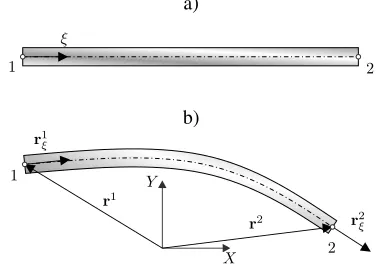
wherer is the global position vector of an arbitrary point on the element, S is the global shape function that depends on the Lagrangian coordinates and eis a vector of time-dependent coefficients that consist of the absolute position and slope coordinates of each node in an element. In this paper a planar gradient deficient [25] Euler-Bernoulli beam element is used [30–32], Fig. 1.
a)
b)
Fig. 1. Position vector and slopes in the planar absolute nodal coordinate beam finite element: a) undeformed and b) deformed reference configuration
The vector of the element nodal coordinatesefor a Euler-Bernoullli finite element is given by
e=e(t) = [e1. . .e8]T. (2) The vector of the nodal coordinates includes the global displacements [4]:
r1=r(0) = [e
1e2]T, r2=r(L) = [e5e6]T, (3)
and the global slopes of the element nodes that are defined as [33]:
r1 x=∂r
1(0)
∂x = [e3e4] T,r2
x=∂r 2(L)
∂x = [e7e8] T. (4)
For this element the shape functionSis a 2×8 matrix and is defined as [25]:
S= [S1I S2I S3I S4I]T, (5) whereIis a 2×2 identity matrix andS1. . .S4can be written as [34]:
S1=1−3ξ2+2ξ3, S2=lξ−2ξ2+ξ3, S3=3ξ2−2ξ3, S4=l−ξ2+ξ3, (6) whereξ =x/Lis the only coordinate of the element with lengthL. Only one gradient vector can be defined at the node and the shear strain is assumed to be zero. As a consequence, the cross-section is assumed to remain perpendicular to the element’s center line.
1.1 Multibody Dynamics
The virtual work of the external forceFjapplied at an arbitrary pointPdefined by the coordinatesxPj on the
j-th finite element can be written as [1] and [29]:
δWj e =Fj
T
δrPj =Fj T
Sjxj P
δej=QjT
e δej. (7)
For example, the virtual work Eq. (7) due to the distributed gravity of the finite element can be obtained using the shape function, Eq. (5) as:
δWgj =
j
V [0 −ρg]S
jδej, (8)
δWj
g = −mejg
0 1 2 0
L 120
1
2 0 −
L 12
δej.(9)
The gravitational force vector acting at the element nodal coordinates can be expressed as:
Qj
g=−mejg
0 1
2 0
L 12 0
1
2 0 −
L 12
T
. (10)
1.2 Equations of Motion
A mechanical system is an assembly of rigid and deformable bodies that are connected with kinematic constraints to achieve the design requirements [1]. The kinematic constraint equations that describe the mechanical joints between the bodies as well as time-dependent, user-defined motion trajectories are defined in terms of the vector of generalized coordinates of the system,q, and timetas:
C(q,t) =0, (11) whereC is the vector of constraint equations. The vector q includes the generalized coordinates of the rigid and flexible bodies of the system, where flexible bodies are described with the absolute nodal coordinates vector e. The constraint forces are included in the equations of motion with the use of Lagrange multipliers and the equations of the system have the form:
Mq¨=Qe−Qs−CTqλ, (12) whereMis a symmetric mass matrix of the multibody system and includes rigid and deformable bodies, Cq is the Jacobian matrix of kinematic constraints Cq =∂C/∂q, ¨q is the vector of accelerations of the multibody system, Qe is a vector of all the applied external forces, including the contact forces, spring forces and gravitational forces,Qsis a vector of elastic strain forces developed only for the deformable bodies, andλ is the vector of Lagrange multipliers. Eq. (12) and the second time derivative of Eq. (11) can be written together in the augmented form [25]:
M CT
q Cq 0
¨ q
λ
=
Q
e+Qg−Qs
Qd
, (13)
whereQd is the vector that absorbs all the terms of the acceleration constraint equations that depend only
on the velocities [35]. The vector of accelerations ¨q can then be integrated forward in time to obtain the velocities ˙qand coordinatesq[36].
For the i-th deformable body (that is assembled from ne number of ANCF finite elements) the mass matrix and the force vectors are presented in details in Section 4 [25].
The effect of pre-stress is introduced to the rigid or ANCF flexible body with the external force applied to the flexible body using Eq.(7) and the force magnitude and direction must be defined, although this rapidly decreases to zero during the time integration.
2 THE NUMERICAL MODEL OF A PRE-STRESSED RIGID-FLEXIBLE ASSEMBLY
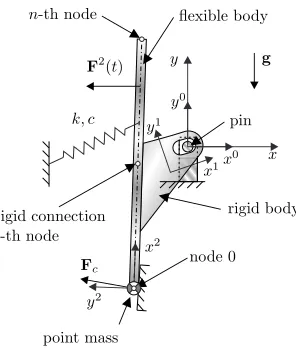
A real mechanical system of a pre-stressed rigid-flexible assembly of a residual current circuit breaker (RCBO) is used in the experimental setup, Fig. 2, and also for the numerical model’s validation, Fig. 3. The mechanical system is assembled from an inertially fixed pin, a rigid body, a point mass, a flexible body and a pre-stressed helical compression spring. The helical compression spring is mounted between the inertially fixed housing and the flexible body. The rigid body with a slot is in contact with the pin via a pin-slot clearance joint [37]. An electric cable connects the terminal with the flexible body and if the flexible body is in contact with the static contact the circuit breaker is switched ON and conducts an electric current.
The assembly’s pre-stressed state results from the accumulation of the potential energy in the pre-stressed helical springs and the elastic strain energy in the flexible body. To speed-up the electrical switch, the potential energy due to the pre-stress is used. Details about the numerical model are presented next.
2.1 Numerical Model
An inertially fixed rigid pin body is connected to a rigid slot body with a pin-slot clearance joint [37]. The moving contact part is modeled as three separate bodies, e.g., a rigid slot body, a contact pad as a mass point and a flexible body as a beam based on ANCF. In Fig. 3 the flexible beam is modeled with two ANCF finite elements and three nodes, e.g., i=1 and n =2. The rigid connection is used to mechanically couple the rigid slot body and the flexible body [38]. A pre-stressed helical compression steel spring is attached between the flexible beam body and the ground [35]. The body coordinate system marked with the upper-script number of the body coincides
with a body center of mass for the rigid body, while the body coordinate system for the flexible body is positioned at the first node of a body’s mesh.
At the initial position of the moving contact different forces are applied to keep it in a stationary position, e.g., the force of a helical compression spring, the contact force between a pin and a slot, the pre-stressed contact force between a moving contact and a fixed contact, Fc, and the external pre-stressed force F2(t). The flexible body vibrates continuously under gravity if there is no damping. During a dynamical simulation only the spring force is continuous and the contact force between the pin and the slot is present when the contact is detected.
Fig. 2.A pre-stressed rigid-flexible assembly with contact conditions - the experimental setup
Fig. 3.A pre-stressed rigid-flexible assembly with contact conditions - the dynamical model
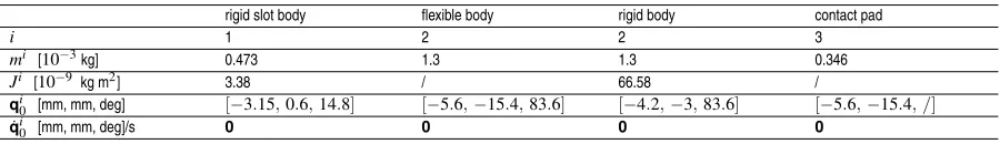
The geometrical and mass properties used for the numerical model of the multibody system are summarized in Table 1. The initial position and the orientation values of the i-th body are marked asqi
0 and the initial velocity vector, ˙qi
0, of the multibody system is zero. The vectorq2
0for the flexible body only defines the position and the orientation of the body’s local coordinate system, which is used to transform the absolute nodal coordinate of the flexible body, while the actual values depend on the number of ANCF finite elements used, e.g., for 2 Euler-Bernoulli ANCF finite elements the vectorq2
0has 3 nodes and each node has 2 vectors (one position and one gradient vector), which in total equals 12 components of the vectorq2
0. A helical compression spring is attached to the housing (ground) at positionus
P=
0,us P,y
and onto the body 2. For a flexible body (i=2) the spring position is defined asL2=18.5 mm, see Fig. 3, and for a rigid body (i=2) the spring position isu2P= [6.5,0.] mm.
Dynamical simulations of the numerical model are performed with custom-written software [39], which automatically generates the equations of motion and uses numerical integration techniques to solve them, Eq. 12.
2.2 Free-Free Response of the Rigid-Flexible Assembly In order to validate the equivalent geometry and stiffness properties of the rigid-flexible assembly a measurement of the bending natural frequencies was made, Fig. 5. A Polytec PDV 100 vibrometer was used to measure the response of the flexible part of the assembly; the impact excitation was introduced via a miniature PCB Piezotronics’s impulse hammer model 084A14. The data acquisition was made using a NI 9234 24-bit data-acquisition card with a sampling rate at 51.2 kHz and 512 samples were acquired during the measurement.
In the numerical model (Fig. 4), all the contacts were removed to obtain the free-free conditions and the external forceF0(t) =0,F0
y(t)Twas applied, where F0
y(t)is:
Fy0(t) =
F0 sin
π
tF t
, ift≤tF
0 , (14)
F0=4 N represents the force amplitude for the selected time interval[0, tF =0.1]ms and the simulation end time istn=100 ms.
Table 2 shows the parameters that were used in the model to obtain the natural frequencies
Table 1.Properties of the multibody system
rigid slot body flexible body rigid body contact pad
i 1 2 2 3
mi [10−3kg] 0.473 1.3 1.3 0.346
Ji [10−9 kg m2] 3.38 / 66.58 /
qi
0 [mm, mm, deg] [−3.15,0.6,14.8] [−5.6,−15.4,83.6] [−4.2,−3,83.6] [−5.6,−15.4, /] ˙
qi
0 [mm, mm, deg]/s 0 0 0 0
Fig. 4.A free-free rigid-flexible assembly
[40] at the free-free boundary conditions shown in Table 3. Table 3 compares the ANCF model to the modal analysis results using the commercial software ANSYS (BEAM188 elements) and the experimental results.
Table 2.Properties of a rigid-flexible assembly
Property Value
lengthL[mm] 25 heighth[mm] 1.1 widthw[mm] 5.2 densityρ[kg/m3] 8940 Young’s modulusE[GPa] 127
Table 3.Bending natural frequencies [Hz] of the rigid-flexible assembly at free-free boundary conditions
Exp. ANCF ANSYS 1stbending frequency [Hz] 4600 4724 4971
Error [%] 0 -2.62 -7.46
3 THE EXPERIMENT
The experimental setup is shown in Fig. 2. Two pre-stress contact forces were measured during the experiment: the PCB 218C was used to acquire the change of contact force on one side (the forceF2
x in the model), while the Endevco 2312 was used on the other (the forceFcin the model). The latter was also used to apply the pre-stress via a string, see Fig. 2. Both sensors are charge-type and require a charge
amplifier (Brüel & Kjaer Nexus 2692 was used). When the pre-stress string on the Endevco 2312 side was instantly cut, the static contact forces were taken from the measured dynamic force. The data was acquired with the NI 9234 (24-bit) card at a sampling frequency of 51.2 kS/s per channel.
During the experiment the motion of the rigid-flexible assembly was recorded with a Photron FASTCAM SA-Z high-speed camera. A frame rate of 67200 fps at a resolution of 384×640 pixels was used. Each pixel corresponded to 47µm for the measured assembly. A digital image correlation (DIC) [23] and [41] was applied to the high-speed camera images to obtain the kinematics of the assembly. An image from recorded sequence is presented in Fig. 6.
3.1 Results
The pre-stressed forcesF2
x andFcwere measured when the string was instantly cut and are shown in Table 4.
Table 4.Measured pre-stressed forces
Measured force F2
x [N] 11.77
Fc[N] 2.92
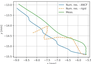
The kinematics of the position vector of node 0 in the x (i.e., e0
x) and y (i.e., e0y) direction obtained from the DIC are shown in Figs. 7 and 8, respectively. Finally, the trajectory of node 0, e0, is shown in Fig. 9. The experimental results are compared to the numerical results obtained using two numerical models: the deformable rigid-flexible assembly presented in Section 2 and a rigid assembly. The rigid assembly was similar to the flexible-rigid assembly, but the "flexible body” (Fig. 3) was modeled as rigid and therefore not able to accumulate the potential energy due to the pre-stress.
Fig. 5.Measurement of bending natural frequencies of the rigid-flexible assembly for free-free boundary conditions
Fig. 6.An image recored with high-speed camera at experiment timet= 0.98 ms
the movement is started. Once the numerical model is partially validated it can be used to research the parameter’s influence. Fig. 10 shows the comparison of thexcoordinate of node 0,e0
x, for different values of
the pre-stress force, the parameter of torsional stiffness
Fig. 7.Axcoordinate of a node0,e0x, on a flexible body and comparison
with a rigid body and experimental values
Fig. 8.Aycoordinate of a node0,e0y, on a flexible body and comparison
with a rigid body and experimental values
ct and the location of the attached helical spring usP,y.
From the results it follows that a doubled pre-stress and a decreased stiffnessctand a change in the attachment
of the helical springus
P,yfrom 0 mm to−1 mm would
Fig. 9.A trajectory of a node0,e0y, on a flexible body and comparison to
a rigid body and measured values
result in 2 mm of distance in approximately 0.6 ms, which is approximately 1/3 of the current switch-off time.
Fig. 10. Axcoordinate of a node0,e0x, on a flexible body for different values of prestress effect
4 CONCLUSIONS
In this work a pre-stressed rigid-flexible dynamical system based on a real mechanical system and a flexible body is modeled with an absolute nodal
coordinate formulation. The dynamical system is
assembled from rigid and flexible bodies that are interconnected with kinematic constraints. First, the bending frequency of the rigid-flexible assembly is measured and based on the measured data an equivalent geometry is designed to achieve equal stiffness properties, including the eigenfrequency. This geometry of the flexible body is then used in a multibody system to model the dynamics and to evaluate the dynamic response of the pre-stressed
rigid-flexible assembly. The dynamics of the
mechanical system is evaluated with digital image
processing of a high-speed camera capture. The
dynamical model is partially validated with the experimental results. The significance of the modeling of flexible bodies in the case of pre-stress is shown.
A good agreement between the measurement and the rigid-flexible model is achieved for x coordinate (Fig. 7) while for the fully rigid assembly model the value of final position is properly simulated. The main difference in the both numerical models is in flexible body and the hybrid rigid connection between rigid slot and flexible body that is achieved with a simple revolute joint with additional torsional spring. For the circuit breaker function theycoordinate is not as important as x coordinate; however it is shown that measured values of yagree well with the numerical values for the rigid-flexible model, while the rigid model gives inappropriate results after time approx. t=1.26 ms, see Fig. 8. The point trajectory of both
numerical models, see table 1, significantly divergate at the end of simulation.
Based on the partially validated numerical model it is clear that a significant decrease in the switch-off time for the electrical contact is possible.
ACKNOWLEDGMENT
The authors acknowledge the partial financial support from the Slovenian Research Agency (research core funding No. P2-0263 and J2-6763).
A APPENDIX
The flexible body can be assembled from multiple ANCF finite elements and evaluated mass matrix and force vectors of the flexible body (continuum) are obtained from mass matrices and force vector of finite elements as [35]:
Mi =
∑
ne j=1Bi jT
Mi jBi j, (15)
Qi
s =
ne
∑
j=1 Bi jT
Qi j
s, (16)
Qi
e =
ne
∑
j=1B i jT
Qi j
e, (17)
whereBi jis a constant Boolean matrix describing the
element connectivity conditions [25]. The Boolean matrix includes zeros and ones and maps the element coordinates to the body coordinates. The Boolean matrix of the finite element always has a number
REFERENCES
[1] Shabana, A.A. (2005). Dynamics of Multibody Systems, Cambridge University Press.
[2] Alankaya, V., Alarçin, F. (2016). Using sandwich composite shells for fully pressurized tanks on liquefied petroleum gas carriers. Strojniški vestnik - Journal of Mechanical Engineering, vol. 62, no. 1, p. 32-40, DOI:10.5545/sv-jme.2015.2611.
[3] Chibueze, N.O., Ossia, C. V., Okoli, J.U. (2016). On the fatigue of steel catenary risers. Strojniški vestnik - Journal of Mechanical Engineering, vol. 62, no. 12, p. 751-756, DOI:10.5545/sv-jme.2015.3060.
[4] Shabana, A.A. (2015). Definition of ANCF finite elements. Journal of Computational and Nonlinear Dynamics, vol. 10, no. 5, p. 054506, DOI:10.1115/1.4030369.
[5] Omar, M.A., Shabana, A.A., Mikkola, A.M., Loh, W.Y., Basch, R. (2004). Multibody System Modeling of Leaf Springs. Journal
of Vibration and Control, vol. 10, no. 11, p. 16011638,
DOI:10.1177/1077546304042047.
[6] Patel, M., Orzechowski, G., Tian, Q., Shabana, A.A. (2016). A new multibody system approach for tire modeling using ANCF finite elements. Proceedings of the Institution of Mechanical Engineers, Part K: Journal of Multi-body Dynamics, vol. 230, no. 1, p. 69-84, DOI:10.1177/1464419315574641.
[7] Čepon, G., Boltežar, M. (2009). Dynamics of a belt-drive system using a linear complementarity problem for the belt-pulley contact description. Journal of Sound and Vibration, vol. 319, no. 3-5, p. 1019-1035, DOI:10.1016/j.jsv.2008.07.005.
[8] Seo, J.-H., Kim, S.W., Jung, I.-H., Park, T.-W., Mok, J.-Y., Kim, Y.-G., Chai, J.-B. (2006). Dynamic analysis of a pantograph-catenary system using absolute nodal coordinates. Vehicle System Dynamics, vol. 44, no. 8, p. 615–630,
DOI:10.1080/00423110500373721.
[9] Gantoi, F.M., Brown, M.A. Shabana, A.A. (2010). ANCF finite element/multibody system formulation of the ligament/ bone insertion site constraints. Journal of Computational and Nonlinear Dynamics, vol. 5, no. 3, p. 031006,
DOI:10.1115/1.4001373.
[10] Langerholc, M., Slavič, J., Boltežar, M. (2013). Absolute nodal coordinates in digital image correlation. Experimental Mechanics, vol. 53, no. 5, p. 807–818, DOI:10.1007/s11340-012-9691-4.
[11] Ayoub, A., Filippou, F.C. (2010). Finite-Element Model for Pretensioned Prestressed Concrete Girders. Journal of Structural Engineering, vol. 136, no. 4, p. 401-409,
DOI:10.1061/(ASCE)ST.1943-541X.0000132.
[12] Akl, A., Saiid Saiidi, M., Vosooghi, A. (2017). Deflection of in-span hinges in prestressed concrete box girder bridges during construction. Engineering Structures, vol. 131, p. 293-310,
DOI:10.1016/j.engstruct.2016.11.003.
[13] Mordak, A., Manko, Z.Z. (2016). Effectiveness of post-tensioned prestressed concrete road bridge realization in the light of research under dynamic loads. Procedia Engineering, vol. 156, no. 264–271, DOI:10.1016/j.proeng.2016.08.296.
[14] Yu, Z., Liu, Y., Tinsley, B., Shabana, A.A. (2015). Integration of geometry and analysis for vehicle system applications: continuum-based leaf spring and tire assembly. Journal of Computational and Nonlinear Dynamics, vol. 10, no. 3, p. 1–17, DOI:10.1115/1.4031151.
[15] Gruber, P.G., Nachbagauer, K., Vetyukov, Y., Gerstmayr, J. (2013). A novel director-based Bernoulli-Euler beam finite element in absolute nodal coordinate formulation free of geometric singularities. Mechanical Sciences, vol. 4, no. 2, p. 279-289, DOI:10.5194/ms-4-279-2013.
[16] Čepon, G., Manin, L., Boltežar, M. (2009). Introduction of damping into the flexible multibody belt-drive model: A numerical and experimental investigation. Journal of Sound and Vibration, vol. 324, ni. 1-2, p. 283-296, DOI:10.1016/j. jsv.2009.02.001.
[17] Rinaldi, R.G., Manin, L., Bonnard, C., Drillon, A., Lourenco, H., Havard, N. (2016). Non linearity of the ball/rubber impact in table tennis: experiments and modeling. Procedia Engineering, vol. 147, p. 348-353, DOI:10.1016/j.proeng.2016.06.307.
[18] Baglioni, S., Cianetti, F., Braccesi, C., De Micheli, D.M. (2016). Multibody modelling of N DOF robot arm assigned to of rows equal to the number of finite element nodal
coordinates and a number of columns equal to the number of nodal coordinates of the flexible body.
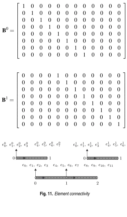
For two ANCF finite elements of Euler-Bernoulli type, as presented in Fig. 11, the boolean matrix of size 8×12 for each element is defined as:
B0=
1 0 0 0 0 0 0 0 0 0 0 0 0 1 0 0 0 0 0 0 0 0 0 0 0 0 1 0 0 0 0 0 0 0 0 0 0 0 0 1 0 0 0 0 0 0 0 0 0 0 0 0 1 0 0 0 0 0 0 0 0 0 0 0 0 1 0 0 0 0 0 0 0 0 0 0 0 0 1 0 0 0 0 0 0 0 0 0 0 0 0 1 0 0 0 0
B1=
0 0 0 0 1 0 0 0 0 0 0 0 0 0 0 0 0 1 0 0 0 0 0 0 0 0 0 0 0 0 1 0 0 0 0 0 0 0 0 0 0 0 0 1 0 0 0 0 0 0 0 0 0 0 0 0 1 0 0 0 0 0 0 0 0 0 0 0 0 1 0 0 0 0 0 0 0 0 0 0 0 0 1 0 0 0 0 0 0 0 0 0 0 0 0 1
Fig. 11.Element connectivity
REFERENCES
[1] A. A. Shabana. Dynamics of Multibody Systems. Cambridge University Press, 2005.
[2] V Alankaya and F Alarçin. Using sandwich composite shells for fully pressurized tanks on liquefied petroleum gas carriers. Strojniški Vestnik/Journal of Mechanical Engineering, 62(1):32–40, 2016.
[3] N. O. Chibueze, C. V. Ossia, and J. U. Okoli. On the Fatigue of Steel Catenary Risers. Strojniški vestnik - Journal of Mechanical Engineering, 62(12):751–756, 2016.
[4] A. A. Shabana. Definition of ANCF Finite Elements. Journal of Computational and Nonlinear Dynamics, 10(5):054506, 2015.
[5] M. A. Omar, A. A. Shabana, A. M. Mikkola, W. Y. Loh, and R. Basch. Multibody System Modeling of Leaf Springs. Journal of Vibration and Control, 10(11):1601–1638, 2004.
[6] M. Patel, G. Orzechowski, Q. Tian, and A. A. Shabana. A new multibody system approach for tire modeling using ANCF finite elements. Proceedings of the Institution of Mechanical Engineers, Part K: Journal of Multi-body Dynamics, 0(0):1–16, 2015.
[7] G. ˇCepon and M. Boltežar. Dynamics of a belt-drive system using a linear complementarity problem for the belt-pulley contact description. Journal of Sound and Vibration, 319(3-5):1019–1035, 2009.
[8] J.-H. Seo, S.W. Kim, I.-H. Jung, T.-W. Park, J.-Y. Mok, Y.-G. Kim, and J.-B. Chai. Dynamic Analysis of a Pantograph-Catenary System Using Absolute Nodal Coordinates. Vehicle System Dynamics, 44(8):615–630, 2006.
[9] F. M. Gantoi, M. A. Brown, and A. A. Shabana. ANCF Finite Element/Multibody System Formulation of the Ligament/Bone Insertion Site Constraints. Journal of Computational and Nonlinear Dynamics, 5(3):031006, 2010.
[10] M. Langerholc, J. Slaviˇc, and M. Boltežar. Absolute Nodal Coordinates in Digital Image Correlation. Experimental Mechanics, 53(5):807–818, 2013. [11] A. Ayoub and F. C. Filippou. Finite-Element
Model for Pretensioned Prestressed Concrete Girders. (April):401–409, 2010.
[12] A. Akl, M. Saiid Saiidi, and A. Vosooghi. Deflection of in-span hinges in prestressed concrete box girder bridges during construction. Engineering Structures, 131:293–310, 2017.
[13] A. Mordak and Z. Z. Manko. Effectiveness of Post-tensioned Prestressed Concrete Road Bridge Realization in the Light of Research under Dynamic Loads.Procedia Engineering, 156:264–271, 2016. [14] Z. Yu, Y. Liu, B. Tinsley, and A. A. Shabana.
Integration of Geometry and Analysis for Vehicle System Applications: Continuum-Based Leaf Spring and Tire Assembly. Journal of Computational and Nonlinear Dynamics, 10(3):1–17, 2015.
[15] P. G. Gruber, K. Nachbagauer, Y. Vetyukov, and J. Gerstmayr. A novel director-based Bernoulli-Euler beam finite element in absolute nodal coordinate formulation free of geometric singularities.Mechanical Sciences, 4(2):279–289, 2013.
[16] G. ˇCepon, L. Manin, and M. Boltežar. Introduction of damping into the flexible multibody belt-drive model: A numerical and experimental investigation. Journal of Sound and Vibration, 324(1-2):283–296, 2009. [17] R. G. Rinaldi, L. Manin, C. Bonnard, A. Drillon,
H. Lourenco, and N. Havard. Non Linearity of the Ball/Rubber Impact in Table Tennis: Experiments and Modeling.Procedia Engineering, 147:348–353, 2016. [18] S. Baglioni, F. Cianetti, C. Braccesi, and D.M.
De Micheli. Multibody modelling of N DOF robot arm assigned to milling manufacturing. Dynamic analysis and position errors evaluation. Journal of Mechanical Science and Technology, 30(1):405–420, 2016. [19] Lionel Manin, Stefan Braun, and Damien Hugues.
Modelling the Belt – Envelope Interactions during the Postal Mail Conveying by a Sorting Machine. Strojniški vestnik - Journal of Mechanical Engineering, 62(7-8):463–470, 2016.
– envelope interactions during the postal mail conveying by a sorting machine. Strojniški vestnik - Journal of Mechanical Engineering, vol. 62, no. 7-8, p. 463-470, DOI:10.5545/sv-jme.2016.3770.
[20] Wolfsteiner, P., Pfeiffer, F. (2000). Modeling, simulation, and verification of the transportation process in vibratory feeders. Journal of Applied Mathematics and Mechanics - Zeitschrift für Angewandte Mathematik und Mechanik, vol. 80, no. 1, p. 35-48, DOI:10.1002/(SICI)1521-4001(200001)80:1<35::AID-ZAMM35>3.0.CO;2-X.
[21] Bayoumy, A.H., Nada, A.A., Megahed, S.M. (2014). Methods of modeling slope discontinuities in large size wind turbine blades using absolute nodal coordinate formulation. Proceedings of the Institution of Mechanical Engineers Part K-Journal of Multi-Body Dynamics, vol. 228, no. 3, p. 314-329,
DOI:10.1177/1464419314528319.
[22] Čepon, G., Manin, L., Boltežar, M. (2011). Validation of a flexible multibody belt-drive model. Strojniški vestnik - Journal of Mechanical Engineering, vol. 57, no. 7-8, p. 539-546,
DOI:10.5545/sv-jme.2010.257.
[23] Langerholc, M., Slavič, J., Boltežar, M. (2013). A thick anisotropic plate element in the framework of an absolute nodal coordinate formulation. Nonlinear Dynamics, vol. 73, no. 1-2, p. 183-198, DOI:10.1007/s11071-013-0778-y.
[24] Shabana, A.A. (1998). Computer implementation of the absolute nodal coordinate formulation for flexible multibody dynamics. Nonlinear Dynamics, vol. 16, no. 3, p. 293-306,
DOI:10.1023/A:1008072517368.
[25] Shabana, A.A. (2008). Computational Continuum Mechanics. Cambridge University Press, Cambridge, DOI:10.1017/
cbo9780511611469.
[26] Shabana, A.A. (1996). Finite element incremental approach and exact rigid body inertia. Journal of Mechanical Design, vol. 118, no. 2, p. 171-178, DOI:10.1115/1.2826866.
[27] Nachbagauer, K., Gruber, P., Gerstmayr, J. (2013). A 3D shear deformable finite element based on the absolute nodal coordinate formulation. In: Samin, J.C., Fisette, P. (eds.) Multibody Dynamics. Computational Methods in Applied Sciences, vol. 28, p. 77-96, Springer, Dordrecht,
DOI:10.1007/978-94-007-5404-1_4.
[28] Gerstmayr, J., Irschik, H. (2008). On the correct representation of bending and axial deformation in the absolute nodal coordinate formulation with an elastic line approach. Journal
Journal of Sound and Vibration, vol. 243, no. 3, p. 565-576,
DOI:10.1006/jsvi.2000.3416.
[30] Escalona, J.L. (1998). Co-ordinate formulation to multibody system dynamics. Journal of Sound and Vibration, vol. 214, p. 833-851, DOI:10.1006/jsvi.1998.1563.
[31] Berzeri, M., Shabana, A.A. (2000). Development of simple models for the elastic forces in the absolute nodal co-ordinate formulation. Journal of Sound and Vibration, vol. 235, no. 4, p. 539-565, DOI:10.1006/jsvi.1999.2935.
[32] Maqueda, L.G., Shabana, A.A. (2009). Numerical investigation of the slope discontinuities in large deformation finite element formulations. Nonlinear Dynamics, vol. 58, no. 1-2, p. 23-37,
DOI:10.1007/s11071-008-9458-8.
[33] Shabana, A.A. (1997). Definition of the slopes and the finite element absolute nodal coordinate formulation. Multibody System Dynamics, vol. 1, no. 3, p. 339-348, DOI:
[34] Shabana, A.A., Hussien, H., Escalona, J.L. (1998). Application of absolute nodal coordinate formulation to large rotation and large deformation problems. Journal of Mechanical Design, vol. 120, no. 2, p. 188-195, DOI:10.1115/1.2826958.
[35] Shabana, A.A. (2009). Computational Dynamics, 3rd Edition.
Wiley, Chichester.
[36] Hussein, B., Negrut, D., Shabana, A.A. (2008). Implicit and explicit integration in the solution of the absolute nodal coordinate differential/algebraic equations. Nonlinear Dynamics, vol. 54, no. 4, p. 283-296, DOI:10.1007/s11071-007-9328-9.
[37] Skrinjar, L., Slavič, J., Boltežar, M. (2016). A validated model for a pin-slot clearance joint. Nonlinear Dynamics, vol. 88, no. 1, p. 131-143, DOI:10.1007/s11071-016-3234-y.
[38] Sugiyama, H., Shabana, A.A. (2004). On the use of implicit integration methods and the absolute nodal coordinate formulation in the analysis of elasto-plastic deformation problems. Nonlinear Dynamics, vol. 37, no. 3, p. 245-270,
DOI:10.1023/B:NODY.0000044644.53684.5b.
[39] Skrinjar, L., Turel, A., Slavič, J. (2016). DyS. From https:// github.com/ladisk/DyS, accesed on 2017-05-04.
[40] Braccesi, C., Cianetti, F., Tomassini, L. (2016). Fast evaluation of stress state spectral moments. International Journal of Mechanical Sciences, vol. 127, p. 4-9, DOI:10.1016/j. ijmecsci.2016.11.007.