R E S E A R C H
Open Access
A novel scheme to design the filter for CT
reconstruction using FBP algorithm
Hongli Shi and Shuqian Luo
**Correspondence: [email protected] School of Biomedical Engineering, Capital Medical University of China, Beijing 100069, China
Abstract
Background: The Filtered Back-Projection (FBP) algorithm is the most important technique for computerized tomographic (CT) imaging, in which therampfilter plays a key role. FBP algorithm had been derived using the continuous system model.
However, it has to be discretized in practical applications, which necessarily produces distortion in the reconstructed images.
Methods: A novel scheme is proposed to design the filters to substitute the standard rampfilter to improve the reconstruction performance for parallel beam tomography. The design scheme is presented under the discrete image model and discrete projection environment. The designs are achieved by constrained optimization procedures. The designed filter can be regarded as the optimal filter for the corresponding parameters in some ways.
Results: Some filters under given parameters (such as image size and scanning angles) have been designed. The performance evaluation of CT reconstruction shows that the designed filters are better than the ramp filter in term of some general criteria. Conclusions: The 2-D or 3-D FBP algorithms for fan beam tomography used in most CT systems, are obtained by modifying the FBP algorithm for parallel beam
tomography. Therefore, the designed filters can be used for fan beam tomography and have potential applications in practical CT systems.
Keywords: Filtered Back-Projection (FBP) algorithm, Computerized tomographic (CT) imaging, Reconstruction, Projection, Optimization
Background
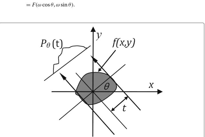
X-ray CT imaging is a procedure to get internal information of an unknown object, such as biological tissue, from the projection data collected by illuminating the object from many different directions using X-ray. The object can be represented by its distribution of X-ray attenuation coefficient. When a parallel beam of X-rays propagates through the object, the total attenuation of the beam can be expressed by a line integral, which is the well-known Radon transform [1,2]
pθ(t)= ∞
−∞f(x,y)δ(xcosθ+ysinθ−t)dxdy,
wheref(x,y)denotes the object (or its distribution of X-ray attenuation coefficient);pθ(t)
denotes the projection data when the scanning angle isθ and the distance between the
projection line and the origin ist;δ(·)denotes the Dirac delta function or the impulse function;xcosθ+ysinθ−trepresents a projection line of X-rays, as shown in Figure 1.
The reconstruction procedure is very important for CT imaging. The properties of the final reconstructed image heavily depends upon the reconstruction algorithm used. Many algorithms have been proposed. They can be roughly divided into three categories: 1) analytical schemes, 2) algebraic reconstruction technique (ART) and 3) statistical iterative reconstruction (SIR) schemes. Some of the ART and SIR algorithms have become hot topics in CT reconstruction research, however, these categories suf-fer from their heavy calculation burden, poor convergence speed and other drawbacks [3-7]. For example, the SIR algorithms lack an efficient stop criterion, and ART algo-rithms are sensitive to noise in the projection data. Both categories of algoalgo-rithms can only been used in a few special fields. The analytical schemes are much simpler and faster. Of these FBP algorithm is the most important one [1,8-11]. FBP algorithm and its modified versions for 2-D and 3-D projection reconstruction, such as FDK (Feldkamp-Davis-Kress) algorithm, have been used in almost all the fields of straight ray tomography, such as X-ray CT and PET (Positron Emission Tomography) [12-14]. The projections can be classified into two types: parallel and fan beam projection. Since the FBP algorithm for fan beam tomography is usually obtained by modi-fying that for parallel beam tomography, only the latter is studied in this paper. The derivation of FBP algorithm for parallel beam tomography is rather simple and straightforward. First, the Fourier slice theorem links 1-D Fourier transform (FT) of the projection data collected at angleθ, Sθ(ω), with 2-D FT at the frequency samples (ωcosθ,ωsinθ ),F(ωcosθ,ωsinθ ). That is
Sθ(ω)= ∞
−∞Pθ(t)exp(−i2π ωt)dt
= ∞
−∞ ∞
−∞f(x,y)exp(−i2π ω (xcosθ+ysinθ ))dxdy =F(ωcosθ,ωsinθ ).
(1)
Then the unknownf(x,y)can be reconstructed by the inverse Fourier transform (IFT) or the dual Radon transform as following
ˆ f(x,y)=
π
0
∞
−∞F(ωcosθ,ωsinθ )|ω|exp(i2π ω(xcosθ+ysinθ ))dωdθ
= π
0
∞
−∞Sθ(ω)|ω|exp(i2π ωt)dωdθ,
where fˆ(x,y) denotes the reconstructed image;t = xcosθ +ysinθ; |ω|is known as
“ramp” filter in the frequency domain. It is well-known thatfˆ(x,y)will be identical with
f(x,y)almost everywhere according to the properties of FT and IFT.
In practice, the projection data and reconstructed images have to be discretized to record, calculate and display. For the discrete projection data,Pθj(l),l∈[−
N
2,· · ·,N2], the
discrete Fourier transform (DFT) and inverse DFT (IDFT) are employed to approximate (continuous) FT and IFT, respectively. They are
Sθj(ω)≈Sθj(k)= N
2−1
l=−N
2
Pθj(l)exp(−i2π
lk
L), k∈[− L
2,· · ·,
L
2] ,
ˆ
f(n,m)≈ π K
K
j=1 Qθj(l),
Qθj(l)= 1
L+1 L
2
k=−L2
Sθj(k)
k L exp
i2πncosθj+msinθjk L
,
(2)
whereNis a positive even integer denotes the number of projection data;Lis an even integer that is equal to or larger than the maximum number of the discrete projection data at all directions;xdenotes the nearest integer ofx;θj,j ∈[1,· · ·,K], denote the discretized scanning angle, andKis the number of the scanning angles. The discretized ramp filter,|kL|, is named as the reconstruction filter in this paper.
For the continuous systems, Radon and inverse Radon transforms are solid and per-fect in the mathematics principle [8-10]. However, it necessarily produces non-negligible degradation when the projection data are discrete (finite) and Radon and inverse Radon transforms have to be discretized in calculation. Many scholars have studied this prob-lem. In [15], a multilevel back-projection method had been presented to improve the computational speed. The point-spread-function (PSF) convolution techniques had been proposed to reduce blurring. By those approaches the image quality was similar with or superior to that using the standard FBP technique. In [16], the spline interpolation and ramp filtering had been combined to improve the standard FBP algorithm, by which the image quality could also be improved somewhat.
2-D DFT of the original image using non-uniform frequency sampling. Then, the recon-structed image is regarded as a convolution of the original image and a particular kernel. The kernel is constructed by 2-D DFT, IDFT and the reconstruction filter to be designed. If the kernel become a 2-D Dirac delta function, the reconstructed image will be identical with the original image. So, the optimal reconstruction filter can be obtained by an opti-mization procedure that make the kernel approach the 2-D Dirac delta function as near as possible.
In order to make the idea behind the design scheme clear, a similar question for 1-D sig-nal is proposed at first, and then it is extended to 2-D situations to solve the corresponding question in CT reconstruction.
Methods
The reconstruction filter for 1-D signal
Suppose a 1-D real signalx(n),n∈[0,· · ·,N−1], whereNis the length of the signal. A special form of DFT is defined as following
X(k)=
N−1
n=0
x(n)exp(−iθkn), k∈[0,· · ·,N−1] , (3)
where θk denoteN angles on the region [0, 2π] correspond toN frequency samples. Similarly, the IDFT is defined as following
ˆ
x(n)= 1 N
N−1
k=0
X(k)exp(iθkn), n∈[0,· · ·,N−1] , (4)
wherexˆ(n)denotes the reconstructed signal.
Ifθk= 2kNπ, (3) and (4) become the standard DFT and IDFT, respectively. It is well-known the original signalx(n)can be perfectly reconstructed when it is transformed into the frequency domain and then transformed back using the standard DFT and IDFT. That is
ˆ
x(n)= 1 N
N−1
k=0
X(k)exp(i2πkn/N)
= 1 N
N−1
m=0 x(m)
N−1
k=0
exp(i2πk(n−m)/N)=x(n).
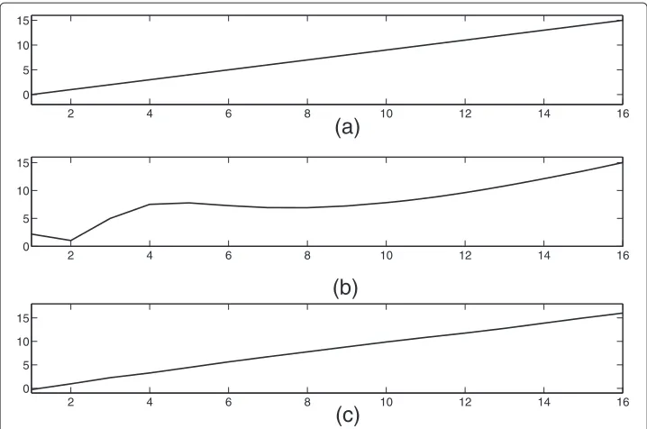
However, it may happenθk= 2Nkπ in some special situations, i.e., the frequency samples do not distribute uniformly in the frequency region [0, 2π]. Whenθk = 2kNπ, the original signal cannot be reconstructed exactly. That is say, the nonuniformity of frequency sam-pling will produce distortion in the reconstructed signal. A simple example is presented to show what will happen when the frequency samples are non-uniform. Suppose the origi-nal sigorigi-nal isx=n,n∈[0, 1,· · ·, 15], which is plotted in Figure 2 (a). It is transformed into the frequency domain and then transformed into the time domain using the frequency samplesθk = (2Nkπ)0.8,k ∈[0, 1,· · ·, 15]. The reconstructed signal is plotted in Figure 2 (b), which is quite different from the original signal.
2 4 6 8 10 12 14 16 0
5 10 15
2 4 6 8 10 12 14 16
0 5 10 15
2 4 6 8 10 12 14 16
0 5 10 15
(c)
(a)
(b)
Figure 2 The original signal and its different reconstructed versions.(a)The original signal,(b)the reconstructed signal after DFT and IDFT usingθk=(2kπ/N)0.8,(c)the reconstructed signal after the identical DFT, IDFT and a filtering process using the designed filter between DFT and IDFT.
pseudo inverse of a large matrix. In order to avoid such a problem, we propose an alternative approach. At first, the reconstructed signal is expressed as following
ˆ
x(n)= 1 N
N−1
k=0
X(k)exp(iθkn)= 1 N
N−1
k=0
N−1
m=0
x(m)exp(−iθkm)exp(iθkn)
= 1 N
N−1
m=0 x(m)
N−1
k=0
exp(iθk(n−m))= N−1
m=0
x(m)h(n−m),
(5)
whereh(n−m)= N1 Nk=−01eiθk(n−m). The reconstructed signal can further be expressed as the periodic (or circular) convolution ofhandx,
ˆ
x=hx, (6)
where denotes the periodic convolution operator; x = [x(0),· · ·,x(N − 1)];
ˆ
x=[xˆ(0),· · ·,xˆ(N−1)];h=[h(−N+1),· · ·,h(0),· · ·,h(N−1)], which is referred to as the convolution kernel.
From (5) or (6), ifh(l)=δ(l), l∈[−N+1,· · ·,N−1], i.e.,
h(l)=δ(l)=
1, l=0, 0, l=0,
thenxˆ(n) = x(n). For example, it can be proven that ifθk = 2kNπ (the standard DFT), it resultsh(l) = δ(l), andxˆ(n) = x(n). It also means the moreh(l)is nearδ(l), the more
ˆ
x(n)is nearx(n).
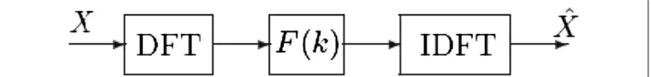
Figure 3. According to (5) or (6),F(k)should be designed to drive the new convolution kernelh(l)= N1 Nk=−01eilθkF(k)to approachδ(l)as near as possible.
Remark 1.From (6), ifh(l) =δ(l), the aliasing distortion will be produced. The more
h(l)is far fromδ(l), the more aliasing distortion will be produced.F(k)acts as a correc-tion term to makeh(l)approachδ(l)as near as possible. However, the residual difference betweenh(l)andδ(l)not only depends onF(·)but also depends on the original kernel
1
N
N−1
k=0 eiθkl. Generally, the difference can be reduced and cannot be removed. The
far-ther the original kernel is different fromδ(l), the more residual difference betweenh(l)
andδ(l)may remain.
Obviously, the convolution kernel may be a complex number. In order to keepxˆ(n)
always as a real number, only the real part of h(l), hr(l) = N1 kN=−01cos(θkl)F(k), is retained in reconstructing the signal. The simplification can also reduce the calculation burden in the designF(k). Since it is unknown and may be very complicated,F(k)has to be expressed in the approximation models, such as Taylor series expansion,
F(k)=
S
n=0
ankn, (7)
whereS is the degree of Taylor series;an denotes the coefficient to be estimated. The coefficient estimation has been achieved by a constrained optimization procedure in this paper. The requirementhr(0) = 1 has been selected as the constrained condition, and
l=0h2r(l) has been selected as the objective function. The constrained optimization problem becomes
min F(k)
l=0
N−1
k=0
cos(θkl)F(k) 2
,
s.t. 1
N
N−1
k=0
F(k)−1=0.
(8)
For the example in Figure 2, selectS=18. Thefminconfunction inOptimization Tool-boxofMatlabis employed in optimizing the nonlinear multivariable objective function (8). The results of optimization procedure, i.e. the coefficients of Taylor series (7) is shown Table 1.
In the example, by insertingF(k),hr(l)is very nearδ(l), which is shown in Figure 4 (b). However, withoutF(k),hr(l)is quite different fromδ(l), which is shown in Figure 4 (a). The objective function in (8) can also be employed as an evaluation criterion. The result
Table 1 The coefficients of Taylor series expansion ofF(k)(N=16,θk=(2πk/N)0.8)
a0 0.001585600279081 a9 0.604131093429063
a1 -0.030192172552822 a10 0.108486066097029
a2 0.213462131921848 a11 -0.404865317972757
a3 -0.686735955366388 a12 -0.674935753170146
a4 1.122118847097341 a13 -0.298926140115388
a5 -0.387130280716676 a14 -0.084322132559712
a6 -0.834889525296690 a15 0.339643128448386
a7 -0.005116780492169 a16 0.662450316746720
a8 0.655962903880333 a17 0.239001712406937
a18 -0.529727742063988
isl=0(161 15k=0cos(θkl)F(k))2 = 0.0013. Without the filtering procedure, the evalua-tion criterion becomesl=0(161 15k=0cos(θkl))2. It resultsl=0(161
15
k=0cos(θkl))2 = 0.2093. A much bigger value means the much more distortion will be brought into the reconstruction signal.
In this paper,F(k)is referred to as the reconstruction filter. It can improve the recon-struction performance significantly, which is illustrated by the same example above. The new reconstructed signal is plotted in Figure 2 (c), which is quite similar with the original signal.
The example illustrates the reconstruction performance can be improved by an addi-tional digital filter designed properly. In the next section, a similar scheme is used in designing the reconstruction filter for CT reconstruction.
The reconstruction filter for CT reconstruction
Letf(n,m)denote the discrete unknown image,n,m∈[−N2,· · ·,N2 −1],Nis a positive even integer. The image is projected on a detector from different scanning anglesθj,j ∈ [1,· · ·K], which produces the projection datapθj(l),l ∈[−L2,· · ·,L2 −1],Lis a positive
−15 −10 −5 0 5 10 15
−0.5 0 0.5 1
−15 −10 −5 0 5 10 15
−0.5 0 0.5 1
(a)
(b)
even integer equals to or is larger than the maximum number of the discrete projection data at all directions. A special 2-D DFT of the image is defined as
Skcosθj,ksinθj
=Sk,θj
=
N
2−1
n=−N2 N
2−1
m=−N2
f(n,m)exp
−i2πkncosθj+msinθj L
, (9)
wherek∈[−L2,· · ·,L2−1].S(kcosθj,ksinθj)can be approximately calculated using the following equation because of projection mechanism.
Sk,θj≈
L
2−1
l=−L
2
pθj(l)exp
−i2πkl
L
. (10)
The reconstructed imageˆf(n,m)can be obtained by the 2-D IDFT ofS(k,θj), which is
ˆ
f(n,m)= 1 LK
K
j=1
L
2−1
k=−L2
Sk,θj
exp
i2kπncosθj+msinθj L
. (11)
By substituting (9) into (11), it results
ˆ
f(n,m)= 1 LK
K
j=1
L
2−1
k=−L2 N
2−1
n=−N2 N
2−1
m=−N2
f(n,m)
·exp i2πk
n−ncosθj+
m−msinθj
L
= 1
LK
N
2−1
n=−N2 N
2−1
m=−N2
f(n,m)
· ⎛ ⎜ ⎝ K
j=1
L
2−1
k=−L2
exp(i2πk(n−n)cosθj+(m−m)sinθj
L ) ⎞ ⎟ ⎠ = N
2−1
n=−N2 N
2−1
m=−N2
fn,mhn−n,m−m.
(12)
where
hn−n,m−m
= 1
LK
K
j=1
L
2−1
k=−L2
exp i2πk
n−ncosθj+(m−m)sinθj
L
. (13)
Considern,n,m,m ∈[−N2,· · ·,N2 −1],h(n−n,m−m)can be regarded as an ele-ment of a matrixH = {h(n−n,m−m)}n,n,m,m. The matrix,H ∈ R(2N−1)×(2N−1), is named as the reconstruction matrix in this paper. The reconstruction procedure (12) can be expressed as following
ˆ
wheredenotes the 2-D periodic convolution operator here;His the 2-D convolution kernel.
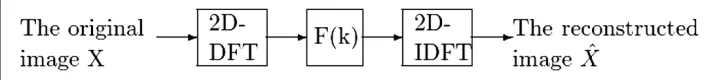
Generally,θj+1−θj= πK is a constant, i.e., the projection angles distribute equally in the region [ 0,π]. However, the frequency samples(2πkLcosθj, 2πkLsinθj)do not distribute equally in the 2-D regions, such as [−π,π]2. Therefore, (9) and (11) form 2-D DFT and IDFT using the non-uniform frequency sampling, and the non-ignorable distortion will be brought into the reconstructed image. This problem is very similar with the 1-D exam-ple in the previous subsection. In order to reduce the distortion, an additional filter is necessary. It is similar withF(k)in Figure 3, and is shown in Figure 5. Further more, the idea behind the design of the additional filter for CT reconstruction is quite similar with that for 1-D signal reconstruction.
Similarly, the design has been achieved by a constrained optimization procedure. From (12) or (14), ifh(n,m)=δ(n,m),fˆ(n,m)=f(n,m). That is say, ifHis aδmatrix (a matrix whose elements all are zeros except that the center element is one), the original image will be reconstructed exactly. It also means the moreh(n,m)is close toδ(n,m), the more
ˆ
f(n,m)is close tof(n,m). Therefore,F(k)should be designed to driveh(n,m)to approach
δ(n,m)as near as possible. Since it is unknown and is perhaps very complicated,F(k)has to be expressed in the approximation models, such as (7) or Fourier series expansion as following
F(k)=a0+
M
m=1
amsin
mkπ
N +bmcos
mkπ N
, (15)
whereMis the degree of Fourier series;amandbmare the coefficients to be estimated. With the additional filterF(k), the element of reconstruction kernel or (13) becomes
h(n,m)= 1 LK
K
j=1
L
2−1
k=−L2 exp
i2πncosθj+msinθj
k L
F(k).
Obviously,h(n,m)usually is a complex number. Similarly, only the real part ofh(n,m),
hr(n,m), is retained to ensurefˆ(n,m)to be a real number. So, the Equation (13) has been simplified as following
hr(n,m)= 1
LK
K
j=1
L
2−1
k=−L2 cos
2πncosθj+msinθj
k L
F(k).
In the design, the requirementhr(0, 0) = 1 (or LK1 kL−=01F(k) = 1) is selected as the constrained condition, andn=0,m=0h2
r(n,m)is selected as the objective function. The
constrained optimization problem becomes
min F(k)
n=0
m=0
⎛ ⎜ ⎝
K
j=1
L
2−1
k=−L2 cos
2πncosθj+msinθj
k L
F(k) ⎞ ⎟ ⎠
2
,
s.t. 1
LK
L−1
k=0
F(k)−1=0.
(16)
Remark 2.From (16), it is obvious thatF(k)depends onN(the image size) andθj(the scanning angles). The images of same size with same scanning process will have a same optimalF(k), vice versa. Generally,F(k)can reduce the difference betweenhr(n,m)and
δ(n,m), however, it cannot remove the difference completely.
Remark 3.From (10), the projection and reconstruction model are relatively simple in this paper. There are many factors are not considered, such as the quantization error (the error that when a pixel is not at any projection line and has to be split between the two nearest projection lines) and projection noise. Even though for such a model, the optimization may be rather complicated and difficult. For example, the objective function is very complicated when the image size is large, and/or the number of projection angles is large.
Results
Example 1.In the example, the size of image is selected asN = 256, the projection anglesθ =[0o, 3o,· · ·, 177o]. In the simulation, the expression of the objective function is very complicated, especially for the objective function. We used some tools inSymbolic Math ToolboxofMatlabin simplifying the procedure. Thefminconfunction in Optimiza-tion ToolboxofMatlabis used in finding the minimum of the objective function. The coefficients for the reconstruction filterF(k)in the form of (15) is shown in Table 2, in whichM=9.
The reconstruction filter can drive the reconstruction kernelhr(n,m)to be very close toδ(n,m), which can be illustrated in Figure 6. In the Figure, the dot curve is the center row (0-throw, orhr(0,m)) ofhr(n,m)using the reconstruction filter designed, while the dash curve is the corresponding row ofhr(n,m)using the ramp filter|k/N|. The dash-dot curve is the corresponding row without a filter, and the solid curve denotes the ideal curveδ(l). It shows the curve using the designed filter is closest to the ideal curveδ(l).
Table 2 The coefficients of Fourier series expansion ofF(k)(N=256,θk=0o,3o,· · ·, 177o) a0 0.122730836679312
a1 0.916483009109464 b1 -0.497982711366623
a2 0.462544582824757 b2 -0.120545376607102
a3 0.128736533815128 b3 0.040355538652453
a4 0.167851665809050 b4 -0.182518259771096
a5 0.315690517777738 b5 -0.094362761222605
a6 0.480769918991562 b6 0.285895915083407
a7 -0.189184291984498 b7 0.563061220832784
a8 -0.335163337055193 b8 -0.086997019632140
−8 −4 0 4 8 −0.2
0 0.2 0.4 0.6 0.8 1 1.2
n
Without a filter Using the filter |k/N| Using the designed filter The ideal curve
Figure 6 The comparison of the 0-throws of reconstruction matrixes with and without the reconstruction filters (N=256,θ=[0o,3o,· · ·,177o]).
Consider the symmetry of the reconstruction matrix, it implies the designed filter can makehr(n,m)be more close toδ(n,m)than the ramp filter.
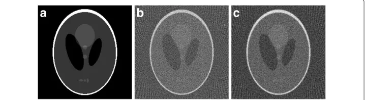
A simulation example is employed to illustrate the availability of the reconstruction filter designed. The original image is of 256×256 pixels,head phantom, which is shown in Figure 7 (a). The projections are calculated usingradonfunction inMatlabwith the rotation angle interval 3o. Since the noise in the projection data are usually modeled by the Poisson distribution [17,18], we suppose the projection data is polluted by Poisson noise whose mean is 5 (also the variance is 5, while the maximum of projection data is 66). It is then reconstructed using FBP algorithm with different reconstruction filters, which are shown in Figure 7 (b) and (c). It shows the small white circle in Figure (c) has more obvious boundary than that in Figure (b).
Three criteria, MSE (Mean Square Error ), UQI (Universal Quality Index) and MI
(mutual information), are employed to assess the efficiency of the designed filter, which are defined as following [19].
MSEfi,f0= 1 M
M−1
k=0
fki−fk02,
wherefkiandfk0denote the pixels of the reconstructed imagefiand reference imagef0, respectively;Mis the total number of pixels in the selected region. Since it is a simulation
Figure 7 The original image and the reconstructed images using FBP algorithm with different reconstruction filters (N=256,θ=[0o,3o,· · ·,177o]).(a)The original image,(b)using the ramp filter
example, the original image is known and selected as the reference image.UQIis defined as following
UQIfi,f0= 2Cov{f
i,f0}
σi2+σ02
2f¯if¯0
¯ fi2f¯02,
wheref¯iandσi2denote the image mean and variance, respectively;Cov{fi,f0}denote the covariance of the reconstructed imagefiand reference imagef0. The mean, variance and
covariance are defined as the following
¯ fi= 1
M
M−1
k=0 fki,
σi2= 1
M−1
M−1
k=0
fki− ¯fi
2
,
Cov{fi,f0} = 1
M−1
M−1
k=0
fki− ¯fi fk0− ¯f0
.
UQImeasures the pixel-to-pixel similarity between the reconstructedfiand reference imagef0. It was designed by modeling any image distortion as a combination of three factors: loss of correlation, luminance distortion, and contrast distortion. Its value ranges between 0 and 1. The closer to 1 theUQIvalue is, the more similar to the reference image the reconstructed image is.
When the reconstructed image and reference image are interpreted as “stochastic processes”,MIis used for measuring their mutual dependence.
MI(fi,f0)=
N−1
k=0
N−1
n=0
p(fki,fk0)log p(f i k,fk0)
p(fki)p(fk0)
,
wherep(fki)andp(fk0)denote the marginal densities offiandf0, respectively, which are calculated using the corresponding histograms; the joint densityp(fki,fk0) is estimated from the joint histogram offi andf0;N denotes the number of bins in the histogram. UQImeasures the pixel-to-pixel dependence of the reconstructed image on the reference image, MI measures the histogram correlation between them.MIcan be highly sensitive to small differences between visually similar images.
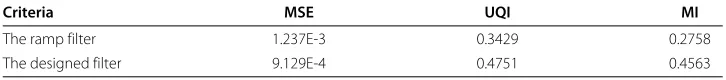
The results for the example in the form of the three criteria are showed in Table 3. The results illustrate the designed filters have better reconstruction performance than the standard ramp filter.
Example 2.In one example, the size of image isN=128×128,θ =[0o, 4o,· · ·, 176o], the coefficients forF(k)in the form of (15) is listed in Table 4. In another example, the size of image isN=256×256,θ =[0o, 1o,· · ·, 179o], the coefficients forF(k)in the form of (15) is listed in Table 5.
Table 3 The results of performance evaluation in Example 1
Criteria MSE UQI MI
The ramp filter 1.237E-3 0.3429 0.2758
Table 4 The coefficients of Fourier series expansion ofF(k)
(N=128,θk=4ko,k=0,· · ·, 44) a0 0.167768278296600
a1 0.742071367715883 b1 -0.050516729362635
a2 -0.007222808863187 b2 -0.257039580419913
a3 0.205121481459339 b3 -0.107883292543924
a4 0.080764672022586 b4 0.021273467611896
a5 -0.013240204304737 b5 -0.106948545272204
a6 0.297619345807562 b6 -0.114131247626016
a7 0.184808294809679 b7 0.324654368672888
a8 -0.198785426563876 b8 0.153168707602131
a9 -0.059263999435747 b9 -0.059403297538579
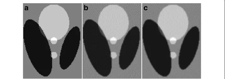
Two similar simulation examples are employed to illustrate the availability of the designed filters. They are thehead phantomof sizes 128× 128 and 256×256 pixels, respectively. The projections are calculated usingradonfunction inMatlabwith the rota-tion angle interval 4oand 1o, respectively. The image is reconstructed using FBP algorithm with different reconstruction filters. The results of performance evaluation in the form ofMSE,UQI andMI are showed in Table 6. The identical small regions of the original image and reconstructed images for the latter example are shown in Figure 8. It shows the artifact has been reduced more efficiently using the designed filter at the interior of white circle and other regions. The results illustrate the designed filters have better performance than the ramp filter for CT reconstruction.
Summary: The simulation examples demonstrate thatF(k)depends on the image size and the projection angles. The images of different sizes and/or with different projection angles usually have different optimalF(k), which makes the problem rather complicated. In order to simplify the expression of reconstruction filter, a much more simple way is to substitute the expression (15) by fitting the filters designed. It is a hyperbolic function as following
F(k)= exp(asin(πk/N))−exp(−asin(πk/N))
exp(asin(πk/N))+exp(−asin(πk/N))
where a is a parameter selected in region [0.5, 2]. For example, a = 1.65 for the
Example1, anda=1 anda=0.6 for the filters inExample2, respectively.
Generally, the more complicated modelF(k) is of, the better properties it has. How-ever, a very much complicated modelF(k)means very much heavy burden of calculation,
Table 5 The coefficients of Fourier series expansion ofF(k)
(N=256,θk=ko,k=0,· · ·, 179) a0 0.209555620787293
a1 0.693546995671764 b1 -0.201010002024803
a2 0.099842536865856 b2 -0.101104690137033
a3 -0.152784751604807 b3 -0.180901677852717
a4 0.248221333497748 b4 -0.353671098582667
a5 0.308013835831055 b5 -0.032248278459190
a6 0.377740474429379 b6 0.104300291184828
a7 0.075385012026711 b7 0.465974969229510
a8 -0.294404584616438 b8 0.114991610901604
Table 6 The results of performance evaluation in Example 2
(Case 1:Size=128∗128,θk=4ko,k=0,· · ·, 44)
Criteria MSE UQI MI
The ramp filter 1.399E-3 0.6454 0.8022
The designed filter 1.229E-3 0.6914 0.8518
(Case 2:Size=256∗256,θk=ko,k=0,· · ·, 179)
Criteria MSE UQI MI
The ramp filter 2.645E-4 0.9219 0.9289
The designed filter 2.415E-4 0.9384 0.9301
which may cause the optimal parameters even the valid parameters cannot be found. On the other hand, the difference betweenhr(n,m)andδ(n,m)can only be reduced and can-not be removed. So a moderate complicated modelF(k), such as (7) withS=18 and (15) withM=9, is an appropriate choice.
Conclusion
For the continuous image model and scanning, FBP algorithm is perfect in the mathematics principle, in which the ramp filter|ω| (it is named as the reconstruction filter in this paper) plays an important role. However, it necessarily causes degradation in the reconstructed images when the continuous image model is discretized and the continuous scanning is substituted by the discrete (finite) scanning in the practical cal-culation. It means the standard discrete version of ramp filter,|k/N|, is not the optimal for the discrete FBP algorithm. In this paper, a novel scheme is proposed to design the new reconstruction filters to substitute the ramp filter. According to analysis, the recon-structed image can be regarded as the 2-D IDFT of 2-D DFT of the original image using non-uniform frequency sampling. It is also equivalent to a 2-D periodic convolution of the original image and a special 2-D kernel (it is named as the reconstruction matrix in this paper). The more the reconstruction matrix is close to aδ-matrix (a matrix whose ele-ments all are zeros except the center element is one), the more the reconstructed image is close to the original image. Therefore, the reconstruction filters are designed to drive the reconstruction matrixes approachδ-matrix as near as possible. The designs are achieved by the constrained optimization procedures. Some simulation examples have been fin-ished. The results demonstrate the filters designed can make the reconstruction matrixes
Figure 8 The small regions of original image and the reconstructed images using FBP algorithm with different reconstruction filters (N=256,θ=[0o,1o,· · ·,179o]).(a)The original image,(b)using general
more close toδ-matrix than the ramp filter. The performance evaluation of CT recon-struction also shows the designed filters have outstanding superiority over the ramp filter in the term of three general criteria, such as MSE, UQI and MI.
Competing interests
The authors declare that they have no competing interests.
Authors’ contributions
Shi carried out all the mathematics analysis, design, simulation, and draft the manuscript. Luo carried out the revision of the spelling, wording, and expression and given some important advices on the framework of the manuscript. Both authors read and approved the final manuscript.
Acknowledgements
This work have been supported by National Natural Science Foundation (NSFC) of China under Grant No. 60972156 and No. 61227802, and Marie Curie International Research Staff Exchange Scheme (IRSES) actions under the 7th Framework Programme of the European Community under Grant No. PIRSES-GA-2009-269124.
The authors greatly appreciate all the anonymous reviewers for their comments, suggestions, questions, even some revisions on language, which helped to improve the quality of this paper.
Received: 6 December 2012 Accepted: 26 May 2013 Published: 1 June 2013
References
1. Kak Avinash C, Slaney M:Principles of Computerized Tomographic Imaging. New York: IEEE Press; 1988. 2. Hsieh J:Computed Tomography-Principles, Designs, Artifacts, and Recent Advances. (Bellingham: SPIE Press) 2003. 3. Lemmens C, Faul D, Nuyts J:Suppression of metal artifacts in ct using a reconstruction procedure that
combines map and projection completion.IEEE Trans Med Imag2009,28:250–260.
4. Jingyan Xu, Taguchi K, Tsui B M W:Statistical projection completion in X-ray CT using consistency conditions.
IEEE Trans Med Imag2010,29:1528–1540.
5. Thibault JB, Sauer K, Bouman CA, Heieh J:A three-dimensional statistical approach to improved image quality for multi slice helical CT.Med Phys2007,34:4526–4544.
6. Sidky EY, Chartrand R, Pan X:Image reconstruction from few views by non-convex optimization.In
IEEE Nuclear Science Symposium Conference Record. Honolulu, HI; 2007:3526–3530.
7. Sidky EY, Pan X:Image reconstruction in circular cone-beam computed tomography by constrained, total-variation minimization.Phys Med Biol2008,53:4777–4807.
8. Faridani A:Introduction to the mathematics of computed tomography.
Inside Out: Inverse Problems, MSRI Publications2003,47:1–46.
9. Natterer F:The Mathematics of Computerized Tomography. Philadelphia: SIAM; 2001.
10. Riedert A, Faridanit A:The semidiscrete filtered backprojection algorithm is optimal for tomographic inversion.SIAM J Numer Anal2003,41:869–892.
11. Ye Y, Wang Q:Filtered backprojection formula for exact image reconstruction from cone-beam data along a general scanning curve.Med Phys2005,32:42–48.
12. Zamyatin AA, Taguchi K, Silver MD:Practical hybrid convolution algorithm for Helical CT reconstruction.
IEEE Trans Nuc Sci2006,53:167–174.
13. Borsdorf A, Raupach R, Flohr T, et al.:Wavelet based noise reduction in CT-images using correlation analysis.
IEEE Trans Med Imag2008,27:1685–1703.
14. Ivakhnenko VI:A novel quasi-linearization method for CT image reconstruction in scanners with a multi-energy detector system.IEEE Trans Nuc Sci2010,57:870–879.
15. Brandty A, Jordan M, Brodskiy M, Galun M:A fast and accurate multilevel inversion Of the radon transform.
SIAM J Appl Math1999,60(2):437–462.
16. Horbelt S, Liebling M, Unser M:Filter design for filtered back-projection guided by the interpolation model.
Proc. SPIE 4684, Medical Imaging 2002: Image Processing, 806 (May 15,2002). [http://proceedings.spiedigitallibrary.org/
proceeding.aspx?articleid=1313610]
17. Xu Q, Yu H, Mou X, et al.:Low-dose X-ray CT reconstruction via dictionary learning.IEEE Trans Med Imag2012,
31(9):1682–1697.
18. Borsdorf A, Raupach R, Flohr T,etal:Wavelet based noise reduction in CT-images using correlation analysis.IEEE
Trans Med Imag2008,27(12):1685–1703.
19. Bian J, Siewerdsen JH, Han X,etal.:Evaluation of sparse-view reconstruction from flat-panel-detector cone-beam CT Phys.Med Biol2010,55:6575–6599.
doi:10.1186/1475-925X-12-50
Cite this article as:Shi and Luo:A novel scheme to design the filter for CT reconstruction using FBP algorithm.