Segmentation of MR image using local and global region based geodesic model

R E S E A R C H

Open Access

Segmentation of MR image using local and global

region based geodesic model

Xiuming Li

, Dongsheng Jiang

, Yonghong Shi

and Wensheng Li

* Correspondence: [email protected]; [email protected] 1

Digital Medical Research Center, School of Basic Medical Sciences, Fudan University, Shanghai 200032, PR China

Full list of author information is available at the end of the article

Abstract

Background:Segmentation of the magnetic resonance (MR) images is fundamentally important in medical image analysis. Intensity inhomogeneity due to the unknown noise and weak boundary makes it a difficult problem.

Method:The paper presents a novel level set geodesic model which integrates the local and the global intensity information in the signed pressure force (SPF) function to suppress the intensity inhomogeneity and implement the segmentation. First, a new local and global region based SPF function is proposed to extract the local and global image information in order to ensure a flexible initialization of the object contours. Second, the global SPF is adaptively balanced by the weight calculated by using the local image contrast. Third, two-phase level set formulation is extended to a multi-phase formulation to successfully segment brain MR images.

Results:Experimental results on the synthetic images and MR images demonstrate that the proposed method is very robust and efficient. Compared with the related methods, our method is much more computationally efficient and much less sensitive to the initial contour. Furthermore, the validation on 18 T1-weighted brain MR images (International Brain Segmentation Repository) shows that our method can produce very promising results.

Conclusions:A novel segmentation model by incorporating the local and global information into the original GAC model is proposed. The proposed model is suitable for the segmentation of the inhomogeneous MR images and allows flexible initialization.

Keywords:Intensity inhomogeneity, Level set method, Local image information, Global image information

Background

Magnetic resonance image can provide excellent spatial resolution and superb soft tissue contrast for anatomical and functional structures. Accurate segmentation of MR image is an essential step in medical image analysis. However, the intensity inhomogeneity due to the unknown noise and weak boundary makes the segmentation a challenge. Various seg-mentation algorithms have been proposed in the literature. Particularly, Active contour model (ACM) receives the widespread attention since it can provide promisingly smooth and closed contours to cover object boundaries with sub-pixel accuracy [1,2]. The exist-ing ACMs can be mainly categorized into two classes: edge-based models and region-based models.

One of the most popular edge-based models is geodesic active contour (GAC) model [3,4], which utilizes image gradient to construct an edge stopping function (ESF) to keep the contour evolution within the object boundaries. The model has been successfully ap-plied in the general images with strong object boundaries, but it may suffer from boundary leakage in the brain MR images which typically contain weak boundaries due to low con-trast and partial volume effect. However, when the initial contour is far away from the de-sired object boundary, the GAC model will fail to find the target [5]. And then Song proposed an edge-based ACM that is driven by the regularized gradient flux flows [6]. The method is not only robust to noise, but also preserves the edge information, thereby achieves accurate segmentation results.

Region-based models have many advantages over the edge-based ones. For example, region-based models are less sensitive to noise and contour initialization since they utilize region information as a substitute for image gradient to constrain contour evolution. Moreover, they can successfully segment images with the weak boundaries or even with-out boundaries. The well-known region-based model, Chan-Vese (CV) model, assumes that image intensities are statistically homogeneous in each region, and therefore it fails to segment MR images with intensity inhomogeneity [7]. Then Li et al. proposed a local bin-ary fitting (LBF) model to overcome the intensity inhomogeneity. The LBF model can provide desirable segmentation results because it uses the mean of the local region infor-mation. However, it is sensitive to the initial contours and is easy to trap into a local mini-mum, which limits their practical applications [8,9]. Zhang et al. proposed a maximum likelihood in transformed domain method to simultaneously segment images and correct bias field. The method demonstrated the superiority by taking the mean and variance in a local region into account [10].

For making full use of the advantage of the three methods mentioned above, some hybrid models combining the local and global intensity fitting energies were proposed to drive the evolution of initial contours. Lei He et al. blended GMM model, Hueckel model and CV model, and finished the segmentation of inhomogeneous image, but is prone to be sensitive to initialization and parameterization [11]. Zhang et al. proposed an improved method of GAC model, named as GCV model, which utilizes the global intensity information to construct a signed pressure force (SPF) function to drive the contour evolution. This method also proposed a new level set function re-initialization method, i.e., selective binary and Gaussian filtering regularized Level Set, which is ro-bust and simple to implement, but is hard to deal with the image having inhomogen-eous gray intensity or weak boundary images [5]. Wang et al. proposed a hybrid level set method which has a LBF term based on the local intensity fitting and CV term based on an auxiliary global intensity fitting. Due to combining the local and global in-tensity information, the proposed model can avoid trapping into a local minimum [12].

level set function to avoid the traditional re-initialization of the level set function to a signed distance function [5]. The proposed model is first presented as a two-phase level set formulation and then extended to a multi-phase formulation. After minimizing the energy function [13], the method is able to segment MR images. Experiments on syn-thetic and MR images show that the proposed method can not only overcome inhomo-geneous gray intensity, but also deal with the images having complex background and weak boundary. Moreover, it reduces function’s dependence on initial contour.

The rest of the paper is organized as follows. We briefly review several classic models and their limitation in “Background”. The proposed method is introduced in “Methods”. We discussed our proposed method and compared our segmentation re-sults with those of GCV method, LBF method and Li et al. method [14] in“Results and discussion”. Finally, some conclusive remarks are included in“conclusion”

The related methods

Given the image I(x),x∈Ωand Ω⊂R2. Let the initial contourC(q):[01]→R2 be a pa-rameterized planar cure in Ω. In this subsection, we will introduce GAC model, CV model, GCV model and LBF, respectively.

The GAC model

The traditional edge-based GAC model [3,4] is formulated as,

EGAC ¼

Z 1

0

gðj∇I C qð ð ÞÞjÞC0ð Þq dq; ð1Þ

wheregis a positive, decreasing and regular edge stopping function (ESF) described as,

gðj j∇IÞ ¼ 1

1þj∇KσIj2; ð2Þ

where∇Kσ*Idenotes convolving imageIwith a Gaussian kernel,Kσ, whose standard deviation isσ. σis the scale parameter that controls the region-scalability from the lo-cally small neighborhood to the whole image domain and is adaptively chosen in the images, similar to [9].

The GAC model utilizes image gradient to construct an edge stopping function (ESF) to stop the contour evolution on the object boundaries. For images of weak boundaries or the initial contour is far away from the desired object boundary, the GAC model will fail to find the target [5].

The CV model

The region-based CV model [7] considered a special case where the original image in-tensity is assumed as homogeneous. The energy function of the segmenting curve Cof CV model is defined as,

ECV _¼λ1 Z

inside Cð Þ

I xð Þ−C1

ð Þ2 dxþλ2

Z

outside Cð Þ

I xð Þ−C2

ð Þ2

dx; x∈Ω; ð3Þ

where C1and C2are two constants which are the average intensities inside and

driven force of the image data inside and outside the contour, respectively. By minimiz-ing Eq. (3)C1andC2are solved as follows:

C1¼

Z

Ω_ZI xð ÞHðϕð ÞxÞdx

ΩHðϕð ÞxÞdx

; ð4Þ

C2¼

Z

Ω_ZI xð Þð1−Hðϕð Þx ÞÞdx

Ωð1−Hðϕð Þx ÞÞdx

; ð5Þ

where ϕ(x) is the level set function andH(ϕ(x)) is the Heaviside function which is regularized as follows:

Hεð Þ ¼z 1

2 1þ

2

πarctanzε

; ð6Þ

where εis nonnegative constant. Similar to [7,8], we set ε=1.0 for good approxima-tion ofHbyHε.

Obviously,C1andC2are related to the global properties of the image contents inside

and outside the contour, respectively. Without taking local image information into ac-count, the CV model fails to segment images with inhomogeneity. Figure 1(a) shows a synthetic image with intensity inhomogeneity. The CV model fails to segment this image, as show in Figure 1(b).

The GCV model

The GCV model [5] utilized the statistics of local region in CV model and proposed a signed pressure force (SPF) function [15] whose value is in the range of [−1, 1]. And GCV can modulate the signs of the pressure forces inside and outside the region of interest so that the contour shrinks when outside the object, or expands when inside the object. The SPF function is defined as follows,

S I xðð ÞÞ ¼ I xð Þ−

C1þC2 2

max I xð Þ−C1þC2 2

; x∈Ω; ð7Þ

whereC1and C2are defined in Eq. (4) and Eq. (5), respectively. Substituting the ESF

in Eq. (1) for the SPF function in Eq. (7), the improved region-based segmentation

(a)

(b)

(c)

(d)

method was formulated as GCV. Figure 2(a) illustrates the interaction of the interior and exterior regions of the contour. The contour curve (green line) divides the image into the interior and the exterior regions of the contour, which are corresponding toC1

andC2computed in Eq. (4) and Eq. (5),respectively.

The GCV model shares the advantages of the CV and GAC models. This model uti-lizes the statistical information inside and outside the contour to construct a region-based SPF function to substitute ESF. Under the effect of SPF function, the contour can shrink when it is outside the object or expand when inside the object. Moreover, the level set function of the GCV model is regularized by the selective binary and Gaussian filtering [5], and the computational complexity is decreased by comparing with the traditional level set methods. However, this method can’t deal with the in-homogeneous or fuzzy boundary images. For example, Figure 1(c) shows that the GCV model fails to segment the object correctly.

The LBF model

The LBF model [8,9] utilizes two spatially varying fitting functionsf1(x) andf2(x) to

ap-proximate the local intensities on the two sides of the contour. And the image fitting energy function was defined as follows:

ELBFðϕ;f1;f2Þ ¼λ1∬Kσðy−xÞðI yð Þ−f1ð Þx Þ 2

Hðϕð Þy Þdy dx

þλ2∬Kσðy−xÞðI yð Þ−f2ð ÞxÞ2ð1−Hðϕð Þy ÞÞdy dx; x∈Ω;

ð8Þ

Due to the localization property of the kernel function, the contribution of the inten-sityI(y) to the LBF energy decreases to zero as the pointymoves away from the center point x. Therefore, the LBF energy is dominated by the intensityI(y) of pointsyin the neighborhood ofx. This localization property plays a key role in segmenting the images with intensity inhomogeneity. Figure 2(b) illustrates the interaction of the local interior and local exterior regions of the point x. The local neighborhood ofx,Kσ(y−x), is rep-resented by the black circle. The circle is spilt by the green curve into local interior (red) and local exterior (green) regions. The small yellow and blue dots represent the

Figure 2Graphical representation of one level set model.The green line denotes the contour curve, which divides the image into two regions, interior regionC1and the exterior regionC2(a). The local neighborhood ofx,Kσ(y−x) is represented by the black circle. The circle is spilt by the green curve into

local interior (red) and local exterior (green) regions. The small yellow and blue dots represent the pointx

along the contour and pointyin the local region of pointx, respectively.f1(x) andf2(x) are computed in the local interior and local exterior region of the pointxto fit the image intensities near the pointx(b).f1(y)

andf2(y) are computed in the local interior and local exterior region of the pointxto fit the image

point xalong the contour and point yin the local region of point x, respectively. f1(x)

and f2(x) are computed in the local interior and local exterior region of the point xto

fit the image intensities near the pointx.

By minimizing Eq. (8),f1(x) andf2(x) are solved as follows,

f1ð Þ ¼x

Z

Kσðy−xÞI xð ÞHðϕð Þy Þdy

Z

Kσðy−xÞHðϕð Þy Þdy

; x∈Ω ð9Þ

f2ð Þ ¼x

Z

Kσðy−xÞI xð Þð1−Hðϕð Þy ÞÞdy

Z

Kσðy−xÞð1−Hðϕð Þy ÞÞdy

; x∈Ω ð10Þ

Because of using local region information, specifically local intensity mean, the LBF model is able to provide desirable segmentation results even in the presence of intensity inhomogeneity. Figure 1(d) shows the correct result of the LBF model. The disadvan-tage of LBF model is that it is easy to fall into a local minimum, and then it is sensitive to the initial location of contour.

Methods

The design of novel SPF function

Our method implements a novel model which combines the advantages of GCV model and LBF model in a new SPF function by simultaneously taking the global and the local intensity information into account. Figure 2(c) shows the main idea of our method. Two fitting functions,f1(y) andf2(y), are computed in the local interior and local

exter-ior region of the point xto fit the image intensities near the point y. In this way, for each center point x, the local SPF function can be minimized when the contourC is exactly on the object boundary. Here, our local SPF function is formulated as,

SLðI xð ÞÞ ¼

Z

Kσðy−xÞ I xð Þ−f1ð Þ þy f2ð Þy

2

dy

max Z

Kσðy−xÞ I xð Þ−f1ð Þ þy f2ð Þy

2

dy

; x∈Ω; ð11Þ

And the global SPF function is equalized toS(I(x)) in Eq. (7),

SGðI xð ÞÞ ¼S I xðð ÞÞ; ð12Þ

Then, our full energy function is formulated as,

SNewðI xð ÞÞ ¼SLðI xð ÞÞ þω⋅SGðI xð ÞÞ; x∈Ω; ð13Þ

whereω balances the local and the global fitting energies. Theoretically, ωshould be set a larger value to make the weight of global SPF function bigger in the regions where intensity varies greatly, while set a smaller one in the regions where intensity varies smoothly. Following the work in [16], we adopt the adaptive weight,

ω¼β⋅CR⋅ð1−CRÞ; ð14Þ

where β is a fixed positive parameter and CR is the average value of CR over the

CRð Þ ¼x

maxðI xð ÞÞ−minðI xð ÞÞ

R R

maxðI xð ÞÞ Ω

whereRdefines the local window of size 5 × 5 centered at x.ω varies between 0 and 1 and reflects how rapidly the intensity changes in a local region. It is smaller in the smooth regions and bigger in the regions close to the boundary of objects. Therefore, theωcan adaptively adjust the global term in all regions.

Eq. (13) indicates thatSNew(I(x)) is in the range of [−1, 1] and can control the contour shrinks when it is outside the object, or expands when inside the object. Accordingly, it satisfies the requirement of being a symbols pressure function. Substituting the ESF in Eq. (1) for the SPF function in Eq. (13), the level set formulation of the proposed model is regularized as following [3]:

∂ϕ

∂t ¼S

New_{ðI xð ÞÞ⋅ div} ∇ϕ

∇ϕ

j jþα

∇ϕ

j j þ∇SNewðI xð ÞÞ⋅∇ϕ; x∈Ω; ð15Þ

whereαis the balloon force, which controls the contour shrinking or expanding.

Extension to multi-phase level set model

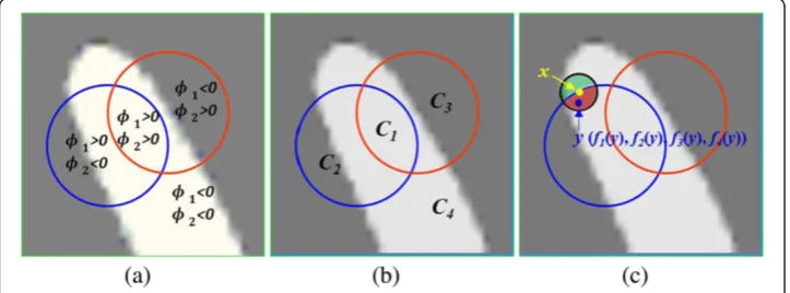
The model proposed above is a two-phase level set formulation, which is not able to segment multiple regions that are adjacent to each other. For example, in brain MR im-ages, the regions of white matter (WM), gray matter (GM), and cerebrospinal fluid (CSF) may be adjacent to each other. An important application of this multi-phase for-mulation is for the segmentation of WM, GM and CSF. Therefore, we extend our model to a phase level set formulation to segment multiple junctions. In multi-phase level set formulation, n level set functions can represent 2n regions [17]. The multi-layer level set formulation can also represent multiple regions [18]. In the study, we focus on four-phase formulation, which is sufficiently to segment brain MR images. Two level set functions,∅1and∅2, are used to define the partition of image domain as

four disjoined regions [17]: {ϕ1> 0,ϕ2> 0}, {ϕ1> 0,ϕ2< 0}, {ϕ1< 0,ϕ2> 0}, {ϕ1< 0,ϕ2<

0}. Let M1=H(ϕ1)H(ϕ2),M2=H(ϕ1)(1−H(ϕ2)),M3= (1−H(ϕ1))H(ϕ2),M4= (1−H(ϕ1))

(1−H(ϕ2)). Figure 3 shows the main idea of our method. The blue and red line denote

the two zero level set function ϕ1 and ϕ2, which divides the image into four regions:

C1,C2,C3andC4in Figure 3(b). The neighborhood of pointx,Kσ(y−x), is represented

by the small black circle and it is spilt by the two level set function into local interior and local exterior regions. The small blue dot represents the pointy in the local region of x. f1(y),f2(y), f3(y),f4(y) are computed in the local interior and local exterior regions

to fit the image intensities near the pointyaccording to the four regions, respectively. Similar to GAC model, energy function is defined as,

E¼α

Z

Ω S

L

1M1þSL2M2þSL3M3

dxþωα

Z

Ω S

G

1M1þSG2M2þSG3M3

dx; ð16Þ

SLi ¼ Z

Kσðy−xÞ I xð Þ−fið Þ þy f4ð Þy

2

dy

max Z

Kσðy−xÞ I xð Þ−fið Þ þy f4ð Þy

2

dy

;i¼1;2;3; x∈Ω; ð17Þ

and the global SPF function,SG

i , is defined as,

SGi ¼ Z

Kσðy−xÞ I xð Þ−CiþC4

2

dy

max Z

Kσðy−xÞ I xð Þ−CiþC4

2

dy

;i¼1;2;3; x∈Ω; ð18Þ

and f1…;f4;C1…;C4 can be similarly derived from Wang et al. [14] paper and Vest

et al. [7] paper.

fið Þ ¼x

Kσð Þ x ½MiI xð Þ

Kσð Þ x Mi ; Ci¼ Z

I xð ÞMidy Z

Midy

; i¼1;2;3;4 ð19Þ

Minimizing the energy functional E in Eq. (16) with respect to ϕ1, we derive the

gradient descent flow:

∂ϕ1

∂t ¼α⋅δ ϕð Þ1 S

L 1−SL3

Hð Þ þϕ2 SL2ð1−Hð Þϕ2 Þ

þω SG

1−SG3

Hð Þ þϕ2 SG2ð1−Hð Þϕ2 Þ

;

ð20Þ

Likewise, minimizing the energy functionalEwith respect toϕ2, we derive the gradient

descent flow:

∂ϕ2

∂t ¼α⋅δ ϕð Þ2 S

L 1−SL2

Hð Þ þϕ1 SL3ð1−Hð Þϕ1 Þ

þω SG1−SG2

Hð Þ þϕ1 SG3ð1−Hð Þϕ1 Þ

h i

;

ð21Þ

whereδ(ϕ) is the Dirac function which is regularized as follows:

Figure 3Graphical representation of two level set model. (a)Blue and red line are considered two zero level set functionϕ1andϕ2, which divides the image into four regions:C1,C2,C3andC4in (b). (c)The neighborhood of pointx,Kσ(y−x), is represented by the small black circle. The circle is spilt

δεð Þ ¼z _π1⋅_ε2þε

z20; ð22Þ

where εis nonnegative constant. if εis too small, the values ofδε(z) tend to be near zero to make its effective range small, so the energy functional has a tendency to fall into a local minimum. The object may fail to be extracted if the initial contour starts far from it. However, if εis large, althoughδ_ε(z) tends to obtain a global minimum, the finial contour location may not be accurate. In“Results and discussion”, we will give some examples to show this drawback. We setε= 0.3 for good approximation ofδbyδ3.

Implementation

We take two-phase segmentation as an example to describe the implementation. In traditional level set methods, the curvature-based term div(∇ϕ/(|∇ϕ|))|∇ϕ| is usually used to regularize the level set function and drive the contour evolution. Instead, Zhang et al. [5] utilizes a Gaussian filter to smooth the level set function for keeping the inter-face and getting rid of the curvature term. In addition, the term, ∇sNew(I(x))⋅ ∇ϕ, in Eq. (15) can also be removed since the model utilizes the statistical information of re-gions, which has a larger capture range and capacity of anti-edge leakage. Finally, the level set formulation of the proposed model, Eq. (15), can be reduced as,

∂ϕ

∂t ¼S

New_{ðI xð ÞÞ⋅αj∇ϕj; x∈Ω; ð23Þ}

The main procedures of the proposed algorithm are summarized as follows: Initialize the level set function∅as:

ϕðx;t¼0Þ ¼

−ρ

0

ρ

x∈Ω0−∂Ω0 x∈ ∂Ω0 ; x∈Ω−Ω0

8 < :

ð24Þ

where ρ> 0 is a constant, Ω0 is a subset in the image domain Ω and ∂Ω0 is the

boundary ofΩ0.

forCheck whether the evolution of the level set function has converged ComputeC1,C2,f1(x) andf2(x) using (4), (5), (9) and (10), respectively.

Evolve the level set function according to Eq. (23). Letϕ= 1 ifϕ> 0; otherwise,ϕ=−1.

Regularize the level set function with a Gaussian filter, i.e.ϕ=ϕ∗Kσ

end

Results and discussion

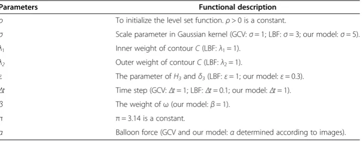
The performance of our method is extensively evaluated in synthetic and real images. Particularly, We first describe the two-phase segmentation which compare the different models, and then show the application of multi-phase segmentation. In addition, the proposed method is implemented in Matlab R2009a on a 2.20GHz PC. Through the whole implementation, the parameters are described in the Table 1.

the global SPF. While in the smooth regions, a biggerω is chosen as the weight of glo-bal SPF so that the contour is attracted to the object boundary quickly. Figure 4(b) is the mask of ω value of a synthetic image and Figure 4(d) is the mask of ω value of a MR image. It can be seen from the two images thatω is bigger in the smooth regions and smaller in the regions close to boundary of objects. Therefore, theωcan adaptively adjust the global SPF term in all regions.

Two-phase segmentation

Our method is first compared with the GCV and LBF model in the synthetic hand and the real blood images whose appearance show severe intensity inhomogeneity. And then our method is also compared in the real MR images to evaluate the performance of our method.

Figure 5 shows that our method can achieve sub-pixel segmentation accuracy. Here, the blue rectangle in Figure 5(a) indicates the initial contour for all methods, and the red contours in (Figure 5(b) and (d)) denote the convergence results by GCV and our model, respectively. The regions surrounded by the green rectangle in (Figure 5(b) and (d)) are zoomed in (Figure 5(c) and (e)), respectively. We can see that our model can deal with intensity inhomogeneity region and the final contour covers the true hand shape, while GCV method make two middle fingers stick together, which is not desired. Here, the parameterαis set to 20.

Figure 6 compares the performance of the LBF and our model in segmenting a real blood vessel image. The vessel image is of intensity inhomogeneity. The second row shows the results of the LBF model. We can see that the LBF can segment intensity Table 1 Description of the parameters used in the study

Parameters Functional description

ρ To initialize the level set function.ρ> 0 is a constant.

σ Scale parameter in Gaussian kernel (GCV:σ= 1; LBF:σ= 3; our model:σ= 5).

λ1 Inner weight of contourC(LBF:λ1= 1).

λ2 Outer weight of contourC(LBF:λ2= 1).

ε The parameter ofH3andδ3(LBF:ε= 1; our model:ε= 0.3).

Δt Time step (GCV:Δt= 1; LBF:Δt= 0.1; our model:Δt= 1).

β The weight ofω(our model:β= 1).

π π= 3.14 is a constant.

α Balloon force (GCV and our model:αdetermined according to images).

(a)

(b)

(c)

(d)

0.025 0.03 0.035 0.04 0.045 0.05 0.055 0.06

0.05 0.1 0.15 0.2

inhomogeneity image on the condition that the initial contour, denoted as yellow rect-angle, lies in the appropriate location such as (Figure 6(a) and (c)). While giving bad initial contour, a bad segmentation result will appear such as the contours indicated by the green arrows in (Figure 6(b), (d) and (e)). On the contrary, the first row shows that our model is less sensitive to the initial contour, and can achieve satisfying segmenta-tion results. Despite the great difference of these initial contours, the corresponding re-sults are almost similar to accurately capture the object boundaries. Furthermore, the iterations and CPU time of segmenting the image with size of 110 × 111 pixels in Fig-ure 6 are listed in Table 2 for LBF model and our method. It can be observed that our method is much faster than LBF model. Accordingly, the proposed method is more ef-ficient. Here, the parameterαis set to 10.

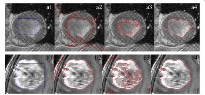
Two MR images with the intensity inhomogeneity shown in (Figure 7(a1) and (b1)) are used to evaluate the proposed model, GCV and LBF model, respectively. Here, the blue rectangles are drawn as the initial contour in (Figure 7(a1) and (b1)). (Figure 7(a2) and (b2)) indicate that the GCV model fails to segment the two images since it is based on only the global intensity information. (Figure 7(a3) and (b3)) show that LBF model

Figure 5Segmenting a hand phantom using the GCV and the proposed model.Illustration of the performance of segmenting a hand phantom (downloaded from [13]) using the GCV and the proposed model:(a)initial contour,(b)segmentation result by the GCV modelα= 20(c)zoomed view of the narrow, green rectangle in (b),(d)segmentation result by our method, and(e)zoomed view of the narrow, green rectangle in(d). The parameterα= 20.

(a)

(b)

(c)

(d)

(e)

is also failed in segmentation of the two images since it uses only the mean of local in-tensity. By contrast, the proposed method incorporating global and local intensity information successfully extracts object boundaries of the two MR images, as shown in (Figure 7(a4) and (b4)).

Multi-phase segmentation of brain MR images

The segmentation of the brain MR images into WM, GM, and CSF is an important task in medical image analysis. A major difficulty in segmentation of MR images is the in-tensity inhomogeneity due to the noise. In this subsection, we will show an application of our multi-phase model to segment brain MR images. We also compare our method with the method of Li et al. [14] on 18 T1-w images obtained from the Internet Brain Segmentation Repository (IBSR) [19].

Frist, we apply our multiphase model to segment two 2D MR images. The initial blue and red contours are displayed in Figure 8(a). The segmentation results of different ε values are shown in Figure 8(b)-(e), respectively. The number of iterations is 50. It can be observed that WM, GM, and CSF are well segmented by our method. From Figure 8 (c) we can see that the tissue and the background of the image can be well-separated, which make our method have a strong discriminative capability for the tissue and the background. In contrast, for the case (b), (d) and (e), the results (Figure 8(b) (d) and (e)) are not consistent with the anatomy of brain in some areas. Such as those pointed by the green arrows. For example, WM is mislabeled as GM in Figure 8(b) and GM is Table 2 Iterations and CPU time (in seconds) needed by our model and LBF model when segmenting the image with the size of 110 × 111 in Figure 6, respectively

Method

Figure6(a) Figure6(b) Figure6(c) Figure6(d) Figure6(e)

Iterations Time(s) Iterations Time(s) Iterations Time(s) Iterations Time(s) Iterations Time(s)

Our model 80 5.36 80 5.17 80 5.23 80 5.26 80 6.18

LBF model 200 12.01 200 13.65 120 8.24 120 8.20 200 14.05

Figure 8Application of our method in segmenting the 3T MR images. (a)original images and initial blue contours,(b) (c) (d) (e)segmentation results ofεis set to 0.1, 0.3, 0.5, 0.8, respectively. The parameterα= 30.

mislabeled as CSF in (Figure 8(d) and (e)). Here,εis set 0.3 in our model and the par-ameterαis set to 50.

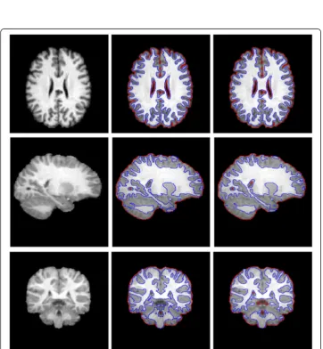
Second, Figure 9 and Figure 10 shows the comparison between the proposed method

and Li’s method. Figure 9 displays the segmentation results by estimating X4

i¼1CiMi.

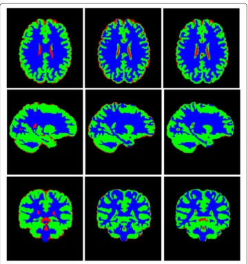
The first Colum in Figure 10 shows the ground truth segmentation from IBSR [19]. It can be observed that the results by our model and Li’s method look similar by visual comparison. We use the Dice Similarity Coefficient (DSC) [20] as an index to measure the segmentation accuracy of WM, GM and CSF, which is defined as

Figure 10Tissue Segmentation masks of Figure8.Colum 1: ground truth; Colum 2: Li’s method; Colum 3: our method.

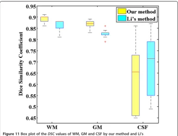
Table 3 The averageDSCvalues of WM, GM and CSF by the two methods, respectively

Tissue WM GM CSF

Li’s method 0.86 ± 0.03 0.83 ± 0.02 0.68 ± 0.14

Our method 0.89 ± 0.01 0.87 ± 0.02 0.63 ± 0.14

DSC Sð 1;S2Þ ¼

2N Sð 1∩S2Þ

N Sð Þ þ1 N Sð Þ2 ; ð25Þ

whereS1and S2represent the obtained segmentation and ground truth, respectively,

and N(·) indicates the number of voxels in the enclosed set. The closer the DSCvalue to 1, the better the segmentation. Table 3 and Figure 11 shows the DSCvalues of WM, GM and CSF by the two methods, respectively. It can be seen that our method can achieve more accurate results by comparing with Li’s method in WM and GM. The third column in Figure 10 shows that our method have a bad performance in segment CSF on the edge of images. So the_DSCvalues of CSF by our method is lower than Li’s method. The p-value of statistical significance of the improvement of our method over Li’s method are less than 0.0005 when using a paired student t-test, which shows that our method significantly outperforms Li’s method with higher accuracy in terms of DSC results. Similarly, compared with Sergi et al. research [21], our method also has relatively high accuracy. Here, the parameterαis set to 100.

Conclusion

This paper presented a novel segmentation model by incorporating the local and global information into the original GAC model. Particularly, a new local SPF function is used to capture the local intensity information, so the novel model is especially fit for the segmentation of the inhomogeneous images. The weight balancing the global term is adaptively adjusted according to the statistics of the local intensity information. In a word, the proposed model can not only allow flexible initialization but also estimate in-tensity inhomogeneity. Moreover, the proposed method has better efficiency since it

reduces the expensive re-initialization of the traditional level set method. In the future, the proposed method will be evaluated in the more extensive experiments.

Competing interests

The authors declare that they have no competing interests.

Authors’contributions

XL developed the algorithm, performed experiments, analyzed the data and drafted the manuscript. DJ provided suggestions and comments. WL participated in the design of the study. YS participated in the algorithm design, coordination and polishing the manuscript. All authors read and approved the final manuscript.

Acknowledgement

This research was supported by the grants from National Natural Science Foundation of Chine grants 60972102, 81271670, 81471758, 81470868, the National High Technology Research and Development Program (2012AA02A606, 2015BAK31B01). This study was also supported by project 12441901600 of Science and Technology Commission of Shanghai Municipality and project 13XD1424800 of 2013 Shanghai Outstanding Technology Leaders Plan.

Author details

1_{Digital Medical Research Center, School of Basic Medical Sciences, Fudan University, Shanghai 200032, PR China.} 2_{Department of Anatomy, Histology and Embryology, School of Basic Medical Sciences, Fudan University, Shanghai}

200032, PR China.3_{Shanghai Key Laboratory of Medical Imaging Computing and Computer-Assisted Intervention,} Shanghai 200032, PR China.

Received: 21 October 2014 Accepted: 12 January 2015 Published: 19 February 2015

References

1. Kass M, Witkin A, Terzopoulos D. Snakes: active contour models. Int J Comput Vision. 1988;1(4):321_–31. 2. Lankton S, Tannenbaum A. Localizing region-based active contours. IEEE Trans Image Process. 2008;17(11):2029–39. 3. Caselles V, Kimmel R, Sapiro G. Geodesic active contours. Int J Comput Vision. 1997;22(1):61_–79.

4. Goldenberg R, Kimmel R, Rivlin E, Rudzsky M. Fast geodesic active contours. IEEE Trans Image Process. 2001;10(10):1467_–75.

5. Zhang K, Zhang L, Song H, Zhou W. Active contours with selective local or global segmentation: a new formulation and level set method. Image Vision Comput. 2010;28(4):668_–76.

6. Song H. Active contours driven by regularised gradient flux flows for image segmentation. Electron Lett. 2014;50(14):992_–4.

7. Chan T, Vese L. Active contours without edges. IEEE Trans Image Process. 2001;10(2):266–77.

8. Li C, Kao C, Gore JC, Ding Z. Implicit active contours driven by local binary fitting energy. In: Proceedings of IEEE Computer Society Conference on Computer Vision and Pattern Recognition (CVPR). 2007. p. 1–7.

9. Li C, Kao C, Gore JC, Ding Z. Minimization of region-scalable fitting energy for image segmentation. I IEEE Trans Image Process. 2008;17(10):1940–9.

10. Zhang K, Liu Q, Song H, Li X. A Variational Approach to Simultaneous Image Segmentation and Bias Correction. 2014.

11. He L, Zheng S, Wang L. Integrating local distribution information with level set for boundary extraction. J Vis Commun Image Represent. 2010;21(4):343–54.

12. Wang L, Li C, Sun Q, Kao C. Active contours driven by local and global intensity fitting energy with application to brain MR image segmentation. Comput Med Imag Grap. 2009;33(7):520–31.

13. Aubert G, Kornprobst P. Mathematical problems in image processing: partial differential equations and the calculus of variations. Springer; 2006.

14. Li C, Huang R, Ding Z, Gatenby J, Metaxas DN, Gore JC. A level set method for image segmentation in the presence of intensity inhomogeneities with application to MRI. IEEE Trans Image Process. 2011;20(7):2007–16. 15. Xu C, Yezzi Jr A, Prince JL. On the relationship between parametric and geometric active contours. In: Proceedings

of the Thirty-Fourth Asilomar Conference on Signals, Systems and Computers, vol. 1. 2000. p. 483–9. 16. Yu Y, Zhang C, Wei Y, Li X. Active contour method combining local fitting energy and global fitting energy

dynamically. In: Proceedings of the International Conference on Medical Biometrics, vol. LNCS 6165. p. 163–72. 17. Vese L, Chan T. A multiphase level set framework for image segmentation using the Mumford and Shah model.

Int J Comput Vision. 2002;50(3):271–93.

18. Chung G, Dinov I, Toga A, LA V. MRI tissue segmentation using a variational multilayer approach, Department of Mathematics, UCLA, CAM Report,08-54. 2008.

19. Internet Brain Segmentation Repository.http://www.nitrc.org/projects/ibsr/.

20. Shattuck DW, Sandor-Leahy SR, Schaper KA, Rottenberg DA, Leahy RM. Magnetic resonance image tissue classification using a partial volume model. NeuroImage. 2001;13(5):856_–76.

21. Valverde S, Oliver A, Cabezas M, Roura E, Lladó X. Comparison of 10 brain tissue segmentation methods using revisited IBSR annotations. J Magn Reson Imaging. 2015;41:93_–101.

doi:10.1186/1475-925X-14-8