A CellML simulation compiler and code generator using ODE solving schemes

R E S E A R C H

Open Access

A CellML simulation compiler and code

generator using ODE solving schemes

Florencio Rusty Punzalan

, Yoshiharu Yamashita

, Naoki Soejima

, Masanari Kawabata

,

Takao Shimayoshi

, Hiroaki Kuwabara

, Yoshitoshi Kunieda

and Akira Amano

Abstract

Models written in description languages such as CellML are becoming a popular solution to the handling of complex cellular physiological models in biological function simulations. However, in order to fully simulate a model, boundary conditions and ordinary differential equation (ODE) solving schemes have to be combined with it. Though boundary conditions can be described in CellML, it is difficult to explicitly specify ODE solving schemes using existing tools. In this study, we define an ODE solving scheme description language-based on XML and propose a code generation system for biological function simulations. In the proposed system, biological simulation programs using various ODE solving schemes can be easily generated. We designed a two-stage approach where the system generates the equation set associating the physiological model variable values at a certain timetwith values att+tin the first stage. The second stage generates the simulation code for the model. This approach enables the flexible construction of code generation modules that can support complex sets of formulas. We evaluate the relationship between models and their calculation accuracies by simulating complex biological models using various ODE solving schemes. Using the FHN model simulation, results showed good qualitative and quantitative correspondence with the theoretical predictions. Results for the Luo-Rudy 1991 model showed that only first order precision was achieved. In addition, running the generated code in parallel on a GPU made it possible to speed up the calculation time by a factor of 50. The CellML Compiler source code is available for download at http://sourceforge.net/projects/cellmlcompiler.

Introduction

In recent years, the continued development in computer processing power paved the way for the increased use of biological function simulation. Computers have proven to be invaluable in analysing complex and nonintuitive biological models and biologists are turning to them to complement their experiments. Simulations enable the testing of experimentally unfeasible scenarios and can potentially reduce experimental costs. However, the num-ber and complexity of physiological models has also grown with the increase in computing performance. This creates challenges in reproducing simulated behaviours of the published models and reuse of models by other researchers, hindering the dissemination of science and knowledge integration.

*Correspondence: fl[email protected]

1Graduate School of Life Sciences, Ritsumeikan University, Shiga, Japan Full list of author information is available at the end of the article

One way to address model complexity is to use markup language-based model descriptions. Some popular exam-ples include CellML [1], SBML (Systems Biology Markup Language) [2] and insilicoML [3]. CellML is an open stan-dard markup language capable of describing mathematical models of cellular functions. SBML is an open interchange machine-readable format for representing models of func-tions such as metabolism and cell signalling. Meanwhile, insilicoML describes mathematical models for biophysi-cal objects and incorporates morphologibiophysi-cal information such as shape, angle and position. SED-ML (Simulation Experiment Description Language) [4] is another type of description language which can encode the informa-tion of simulainforma-tion experiments. These markup languages allow researchers to take advantage of the vast amount of biological function models using a common set of easily readable and versatile description rules.

Biological and physiological function models are gener-ally described by differential equations. A typical simula-tion of biological funcsimula-tion models consists of three parts:

a model equation, a boundary condition, and an ordi-nary differential equation (ODE) solver. Model equations and boundary conditions can be described using CellML, while ODE numerical solutions like Euler and Runge-Kutta methods are typically built into the simulation soft-ware. However, it is necessary to be flexible in using ODE schemes in order to strike a balance between computa-tional stability and speed. In addition, those using special hardware environments such as massively parallel com-puter systems require dedicated proprietary software to support their numerical solution needs. Thus, description languages like CellML and dedicated simulation software are not suitable or practical for flexibly incorporating different ODE solving schemes.

To address the need for more flexibility in creating simulation software, we created Time Evolution Calcu-lation Markup Language (TecML), a machine-readable format for encoding ODE numerical solutions. TecML is a description language based on the extensible markup language (XML). This description language is designed to specify and store the numerical methods that can be used for solving the ODEs in biological models. It also allows the assignment of boundary conditions into the simula-tion experiments. The following secsimula-tions describe TecML and how it is integrated into the proposed code generation system, which automatically generates codes for biological simulations.

The target of this study is limited to the use of different ODE numerical solutions and their application to models described in CellML. We propose an algorithm that allows users to change the ODE solution and boundary condi-tions of the model according to the computational needs of their simulation. To verify the effectiveness of the pro-posed system, we generate executable codes for several CellML models using a number of ODE numerical solu-tions. The system can generate code in several program-ming languages and code that runs in both sequential and parallel computing environments. Simulations on GPU (Graphics Processing Units) were undertaken to show the effect of using parallel computing on processing time.

Biological simulation code generation system Summary of simulation code generation system

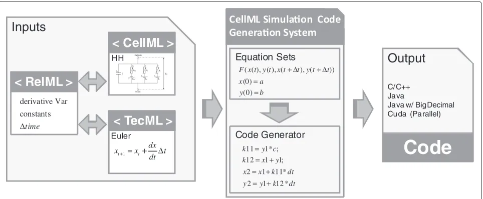
The proposed method is composed of two stages (Figure 1). In the first stage, the system represents the biological model by incorporating an ODE numerical solution method into the model’s differential equations. This creates the equation sets that calculate the time evolution of the mathematical model. The second stage generates the simulation code for these sets of equations, allowing the user to run computer simulations of the model in machines with general-purpose compilers. This approach enables the flexible construction of code gener-ation modules that can support complex sets of equgener-ations.

By generating the code separately for each section of the mathematical model, parallel code execution can be easily integrated into the simulation.

To illustrate the capabilities of the proposed system, we used the FitzHugh-Nagumo (FHN) excitable media model [5] as an example. The model, proposed by R. FitzHugh in 1961 and which J. Nagumo et al. created an equivalent circuit, is a simplification of the Hodgkin-Huxley model and can be described by the following equations:

r=x3, (1)

dx/dt=x−r/3.0−y+a, (2)

dy/dt=b(x+c−d·y), (3)

wherer, xandyare variables,tindicates time anda,b, c,dare constants. Removable algebraic expressions such as equation (1) are often used in biological models to improve the model’s readability.

As for the ODE numerical solution, we used the Mod-ified Euler method to solve the ODEs in (2) and (3). By combining a mathematical description of the model above with the ODE solution method and boundary conditions, we can derive the formula to calculate the time evolution of the independent variablesxandy. This involves finding the solution to the variable vectorξ using its derivatives, temporal variable vectorι, and initial conditions at timet given by

dξ/dt=f(t,ξ,ι), (4)

ι=g(t,ξ). (5)

The rest of this section shows how the proposed sys-tem incorporates the Modified Euler method into the model equations to calculate forξ. The following set of equations represent the numerical solution with boundary conditions:

ξ0=ξt, (6)

t0=t, (7)

ι0=g(t0,ξ0), (8)

κ1=f(t0,ξ0,ι0), (9)

ξ₁=ξ0+κ1·δ, (10)

t1=t0+δ, (11)

ι1=g(t1,ξ1), (12)

κ2=f(t1,ξ1,ι1), (13)

ξ₂=ξ₀+1

2(κ1+κ2)·δ, (14)

ξ_t+δ=ξ₂, (15)

whereξ,κandιare the vectors representing the variables and differential equations in the biological model.

< CellML >

< TecML >

t dt dx x x_t+1= _t+ Δ

< RelML >

Δtime constants derivative Var

Inputs

Code

Java w/ BigDecimal Cuda (Parallel)

Output

Figure 1Code generation system inputs and outputs.Input and output of the Biological Simulation Code Generation System. The inputs are composed of a CellML, TecML, and RelML file. The system can generate simulation codes in C/C++, Java, and Cuda C programming language.

First, from equations (6) and (7), the current values of the differential variables at t are assigned as the initial values with

x0=xt, (16)

y0=yt, (17)

t0=t. (18)

Then with equations (8) and (9), the differential and nondifferential equations are expanded and evaluated using these initial values to obtain

r0=g1(t0, [x0y0]T)=x30, (19)

κ1,x=f1(t0, [x0y0]T,r0)

=x0−r0/3.0−y0+a, (20)

κ1,y=f2(t0, [x0y0]T,r0)

=b(x0+c−d·y0). (21)

Next, the new values ofxandyare computed as func-tions of κ1 and δ (equations (10) and (11)) and given

by

x1=x0+κ1,x·δ, (22)

y1=y0+κ1,y·δ, (23)

t1=t0+δ. (24)

This process is repeated for r1 and κ2 as shown in

equations (12) and (13);

r1=g1(t1, [x1y1]T)=x31, (25)

κ_2,x=f1(t1, [x1y1]T,r1)

=x1−r1/3.0−y1+a, (26)

κ2,y=f2(t1, [x1y1]t,r1)

=b(x1+c−d·y1). (27)

Finally, the value of the differential variables are obtained by advancing the solution from timettot+δ (equations (14) and (15)) with

x2=x0+

1

2(κ1,x+κ2,x)·δ, (28)

y2=y0+

1

2(κ1,y+κ2,y)·δ, (29)

xt+δ=x2, (30)

yt+δ=y2. (31)

The variablerof the equation set corresponds toιwhile x and y are the variables in the vector ξ. The deriva-tives dx/dt and dy/dt are expressed by κ in equations (20), (21), (26) and (27).

In order to automatically incorporate the ODE numer-ical solution into the CellML model, we introduced an ODE solving scheme description language called Time Evolution Calculation Markup Language (TecML). TecML is an XML-based description language that can be used to configure ODE solutions and implement the algo-rithm described in equations (6) – (15). Another input of the system is the Relation Markup Language (RelML) file. The basic role of a RelML file is to relate the variables and variable types of the CellML file into their equivalent in the TecML file.

Description language

The code generation system requires three inputs, namely, the CellML file, TecML file and RelML file. This section gives a short introduction of each and how it is used in the algorithm and consequently, in the FHN model example.

CellML model encoding standard

The CellML [1] language is an open standard based on XML for describing mathematical models. It was designed to allow scientists to share models even if they are using different model-building software. The majority of the models stored in its repository are cell representations and these include information about the cell structure, equations for underlying processes and in some cases, boundary conditions. Figure 2 shows how a CellML model describes the mathematical equations of the FHN cell model. The file lists the input and output variables as well as their initial values and underlying equations. Note that compact syntax representation is used to show its con-tents and is based on Alan Garny’s notation for CellML in the Cellular Open Resource (COR) software [6].

TecML: an ODE solving scheme description language

TecML (Time Evolution Calculation Markup Language) is an XML-based description language designed to describe ODE numerical solutions that can be used in biosimu-lations. This proposed standard allows the mathematical description of solving schemes like the Euler and Runge-Kutta methods. It allows integration of numerical meth-ods with other description languages like CellML. TecML categorizes variables into six different types (Table 1) namely,diffvar,derivativevar,arithvar,constvar,timevar, anddeltatimevar. The variables determined by a rate of change with respect to time (ξ) are referred to as dif-ferential variables (diffvar) while their derivatives (κ) are

Figure 2Information in the CellML file of the FHN model (represented in Alan Garny’s COR notation).

Table 1 Variable and function types in TecML

Type Definition

diffvar Differential variable (variable is a function of time)

arithvar Temporal variable (can be substituted with math equations)

derivativevar Derivative of diffvar

constvar Constants

timevar Time variable

deltatimevar Variable denoting the change of time per step

diffequ Differential equation

nondiffequ Non-differential equation

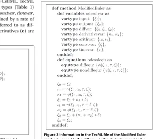
called derivative variables (derivativevar). The removable variables (ι) are the arithmetic variables (arithvar) and variables that do not change in value (ζ) are the constants (constvar). In addition, the time (t) and time increment (δ) are referred to astimevaranddeltatimevar, respectively. TecML also divides the mathematical equations into two types; namely, differential (f()) and non-differential (g()) equations. Equations of type (diffequ) are the derivatives of a function while (nondiffequ) are the arithmetic func-tions. The information and example of a TecML file for the Modified Euler method are shown in Figure 3 and Figure 4, respectively.

Figure 3Information in the TecML file of the Modified Euler method whereξis thediffvar,κis thederivativevar,ζis the

Figure 4TecML file example.

Relation Markup Language (RelML)

RelML is a language for describing the correspondence between the variables in the CellML model file and the variable types in an ODE numerical solution scheme described in a TecML file. Figure 5 shows the corre-spondence of variables described in the FHN CellML file (Figure 2) and the variable types in the TecML file (Figure 3). For the FHN model in Figure 2, variablesxand yare defined as diffvar and their respective derivatives dx/dtanddy/dtasderivativevar. In addition,a,b,c, andd areconstvartype whileris considered a temporal variable orarithvartype. Equations (2) and (3) are the formulas for calculating thediffvarso the functions are categorized as diffequwhile the arithmetic equation forrin equation (1) is anondiffequ.

An example RelML file where the Modified Euler method is applied to the FHN model is shown in Figure 6. The first two statements after the header indicate the filename and location of the corresponding CellML and TecML file. The succeeding lines enumerate all the vari-ables used in the FHN model and their corresponding types. The complete RelML and TecML files used in this paper have been published on the Web [7].

Figure 5Information contained in the RelML file for the FHN model and Modified Euler method.

Figure 6RelML file example for FHN model and Modified Euler method.

Executable code generation for equation sets

The system implementation of the code generator allows the creation of codes in a number of programming lan-guages. Table 2 lists the tested inputs and outputs of the system. For a desktop CPU environment, the gener-ator can produce source codes in C, Java, and Java with BigDecimal library, which can handle higher precision computing. Codes can be generated for both single cell and cell array simulation. The cell array code genera-tor can produce both 1D and 2D excitation propagation codes. The generated codes for 2D simulation describes the excitation propagation in a rectangular array with N × M number of cells. Aside from generating single CPU codes, it can also create codes suited for parallel computing that runs on a GPU machine.

Methods: simulation code generation algorithm Cell model description

The cell model is a collection of variables and equation and can be written as

k=dx/dt=f(x,y,t,z)

y=g(x,y,t,z) , (32)

wherexis a differential variables vector,kis a derivatives vector,yis a temporal variables vector, andzis a constants vector whiletis the scalar variable for time. These variable vectors can be expressed as sets with

x=[x1,x2,· · ·,xNx]

T_{, (33)}

k =[k1,k2,· · ·,kNx]

T_{, (34)}

y=[y1,y2,· · ·,yNy]T, (35)

z=[z1,z2,· · ·,zNz]

T_{, (36)}

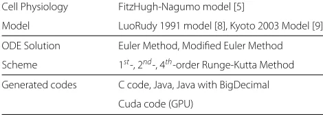
Table 2 Input and output code types in the system

Cell Physiology FitzHugh-Nagumo model [5]

Model LuoRudy 1991 model [8], Kyoto 2003 Model [9]

ODE Solution Euler Method, Modified Euler Method

Scheme 1st_{-, 2}nd_{-, 4}th_{-order Runge-Kutta Method}

Generated codes C code, Java, Java with BigDecimal

where Nx,Ny,Nz are the variable count fork, y, and z, respectively. Furthermore, f(x,y,t,z) andg(x,y,t,z) are function vectors withki=fi(x,y,t,z)andyi=gi(x,y,t,z). These function vectors are defined by

f(x,y,t,z) = [f1(x,y,t,z),· · ·,fNx(x,y,t,z)] T_{, (37)}

g(x,y,t,z) = [g1(x,y,t,z),· · ·,gNy(x,y,t,z)]T. (38)

ODE solving scheme

Table 3 shows the elements inside a TecML file. Note that all the TecML variables are denoted with Greek let-ters. The differential equations for the cell model are represented by the termsdξ/dt = (ξ,ι,t,ζ) andι = (ξ,ι,t,ζ). Inside a TecML file, the dependence between the differential variablesξ0(timet) andξNξ (timet+δ) is given by

ξ_i=σ_i( ,,δ) (0≤i≤Nξ), (39)

κi+1=(ξi,ιi,τi,ζ) (0≤i≤Nξ), (40)

ι_i=(ξ_i,ι_i,τ_i,ζ) (0≤i≤Nξ), (41)

τi=Ti(t,δ) (0≤i≤Nξ), (42)

where the differential variable vector and derivative variable vectorare given by

=[ξ₀,ξ₁,· · ·,ξ_N ξ]

T_{, (43)}

=[κ₁,κ₂,· · ·,κ_Nξ]T. (44)

CellML and TecML integration

The integration of the CellML model and TecML solving scheme involves the mapping of corresponding variables.

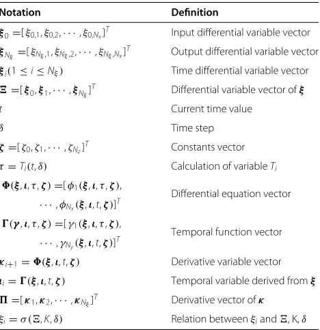
Table 3 Information written in a TecML file

Notation Definition

ξ₀=[ξ0,1,ξ0,2,· · ·,ξ0,Nx]T Input differential variable vector

ξ_Nξ =[ξNξ,1,ξNξ,2,· · ·,ξNξ,Nx]T Output differential variable vector

ξ_i(1≤i≤Nξ) Time differential variable vector =[ξ₀,ξ₁,· · ·,ξ_Nξ]T _{Differential variable vector ofξ}

t Current time value

δ Time step

ζ=[ζ0,ζ1,· · ·,ζNz]T Constants vector

τ=Ti(t,δ) Calculation of variableTi

(ξ,ι,τ,ζ)=[φ1(ξ,ι,τ,ζ), · · ·,φNx(ξ,ι,t,ζ)]T

Differential equation vector

(γ,ι,τ,ζ)=[γ1(ξ,ι,τ,ζ),

· · ·,γNy(ξ,ι,t,ζ)]T

Temporal function vector

κi+1=(ξ,ι,t,ζ) Derivative variable vector ιi=(ξ,ι,t,ζ) Temporal variable derived fromξ

=[κ1,κ2,· · ·,κNξ]T Derivative vector ofκ

ξi=σ (,K,δ) Relation betweenξiand, K,δ

The mapping shows how each physiological model vari-able written in CellML is replaced with its correspond-ing TecML variable. The differential variable vectorξ of TecML corresponds to the differential variable vectorxof CellML and reads as

ξ_k ←xk=[xk,1,xk,2· · ·xk,Nx]

T_{. (45)}

TecML’s derivative variable κ equates to the CellML’s derivative variabledx/dtand the temporal variableι cor-responds toyand given by

κ_k+1←dxk/dt=

dxk,1

dt , dxk,2

dt ,· · ·, dxk,Nx

dt T

, (46)

ι_k ←y_k=[yk,1,yk,2,· · ·,yk,Ny]

T_{. (47)}

Furthermore, the TecML equationsκ=(ξ,ι,t,ζ)and ι=(ξ,ι,t,ζ)correspond to the CellML equationsf and g, respectively, as shown by

(ξ,ι,τ,ζ)←f(x,y,t,z), (48)

(ξ,ι,τ,ζ)←g(x,y,t,z). (49)

Replacement algorithm

Once the variables are mapped, the differential and arith-metic equations are transformed and expanded according to the numerical method described in the TecML file. First, the variables in the CellML model equations are replaced with their corresponding TecML variables. Each model equation is searched for anydiffvar,derivativevar, arithvar,constvar,timevar, ordeltatimevarand that vari-able is replaced with the corresponding TecML varivari-able name. This replacement procedure is represented in Stra-chey brackets and expressed by the following function:

Rvequ=RxRkRyRtRzRdequ,

(50)

where equ is the TecML equation and, for all i = 1, 2, ...,Nξ, the replacement functions are

Rxξi=xi, (51)

Rkκi=ki, (52)

Ryιi=yi, (53)

Rtτi=ti, (54)

Rzζ=z, (55)

Rdδ=d. (56)

Note that the Strachey brackets inRxξi=ximeans that all the TecMLdiffvar(i.e.fori=1. . .Nξ) in the argu-ment is replaced with the corresponding CellMLdiffvar

xi. This function is true for all the other variable types in TecML.

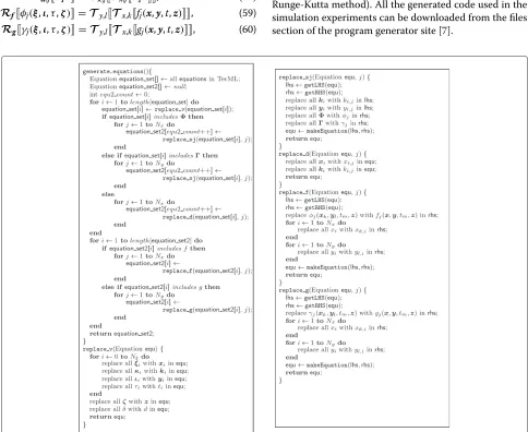
Figure 7 shows how the algorithm generates the simula-tion program from the input files. Note that the

subrou-tinereplace v()in the algorithm replaces variables in

the CellML model equation with the TecML variables as expressed in equation (50). The functionreplace sj()

generates one scalar equation from a vector equation and appends indexjto the variables. In the equations which do not contain functions f or g, replace d() gener-ates multiple scalar equations from a vector equation. Finally,replace f() andreplace g()unfold func-tions f and g, respectively. These subroutines can be expressed in the following transformations:

Rs,jequ=makeEquationSy,jSk,jgetLHSequ,

Sg,jSf,jgetRHSequ,

(57)

Rd,jequ=Sk,jSx,jequ, (58)

Rfφj(ξ,ι,τ,ζ)=Ty,lTx,kfj(x,y,t,z), (59)

Rgγj(ξ,ι,τ,ζ)=Ty,lTx,kgj(x,y,t,z), (60)

where the index-appending functions S and unfolding functionsT are defined as

Sx,jxi=xi,j, (61)

Sy,jyi=yi,j, (62)

Sf,j=φj, (63)

Sg,j=γj, (64)

Tx,kx=xk, (65)

Ty,ky=yk. (66)

Experiments and results

Code generation for the cell model simulation

The FHN cell model [5] was used to evaluate the proposed system. The system was also used to generate simulation codes for a number of cell models (LuoRudy1991 [8], Luo-Rudy1994 [10] and KyotoModel2003 [9]) and with other more accurate ODE numerical methods (e.g. 4th-order Runge-Kutta method). All the generated code used in the simulation experiments can be downloaded from the files section of the program generator site [7].

The traditional approach to creating simulation exper-iment codes also offers little flexibility once the soft-ware is created. Changing the numerical ODE solution method means making major revisions in the simulation code. The proposed method allows the flexibility of using different simulation models, boundary conditions, and numerical methods for a simulation experiment. Since the simulation codes are generated automatically, users can choose or change their desired ODE solver without making changes in the simulation codes themselves. Also, this can give clear information on what is calculated to generate the simulation results.

The different cell models and ODE numerical methods produced varying simulation code sizes. Table 4 lists the number of execution steps generated for the cell models using different ODE solutions. The table shows that the more complex the model becomes and the more equations it has, the larger the number of steps to compute the model equations in the code.

An issue in approximating ODE solutions is the accu-racy of the numerical method used. A good approxima-tion to the underlying differential equaapproxima-tion needs to be achieved in order to arrive at accurate simulation results. We tested a number of commonly used ODE numerical methods to determine how the use of different solutions affect the accuracy of the calculations. The three methods used were Euler, Modified Euler and 4th-order Runge-Kutta. Each of these methods were used to generate an FHN model simulation code that runs in a single CPU. The generated code can run in different compilers and does not require third party software.

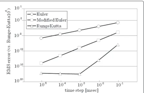
In order to test the accuracy of the ODE numerical methods, simulation codes were generated in Java using the BigDecimal class and numeric formatting. The Java BigDecimal can represent a large number of decimal places and help avoid rounding errors. It can offer higher precisions than the 16 decimal digits offered by floating pointdouble. In the simulation codes, we used BigDeci-mal to represent the numbers in a 32-digit deciBigDeci-mal point precision format for all the ODE solving methods. Differ-ent time steps were also used in testing the accuracy of these ODE methods, ranging from 10−1ms to 10−5ms. The simulation using a time step of 10−6and Runge-Kutta

Table 4 The number of execution steps for the generated codes for different cell models and ODE numerical methods

Cell Model Euler Modified Euler Runge-Kutta

FHN 11 16 26

LuoRudy1991 70 117 211

LuoRudy1994 123 211 387

Kyoto Model 335 560 1200

as ODE solving scheme was used as the basis to com-pute for the root-mean-square error (RMSE) and evaluate the accuracy of the other calculations. The RMSE was computed for all the calculations using different ODE numerical methods and in varying time steps (Figure 8). Each level in the RMSE indicates a 1/10 less accuracy in the simulation results compared to the calculations using Runge-Kutta and 10−6ms time step.

The first-order Euler method gave the largest error (log error≈ 10−3) while the Modified Euler resulted to a smaller error. The fourth-order Runge-Kutta method resulted with the best accuracy (log error≈10−10). How-ever, the Runge-Kutta error is almost constant from the time step 10−3ms, . This can be attributed to the rounding error of digits over the used 32-digit precision.

Simulation codes using different ODE numerical meth-ods were also generated for models more complicated than the FHN or Hodgkin-Huxley model. For this, we used the model introduced by C. Luo and Y. Rudy in 1991 [8]. It is a simple cell model of cardiac action poten-tial that uses Hodgkin-Huxley type equations to calculate ionic currents. The RMSE computations undertaken for the FHN model were also applied for the Luo-Rudy 1991 simulations. Codes were generated for the three ODE solutions with time steps ranging from 10−1to 10−4ms. Meanwhile, the simulation using the Euler method with a time step of 10−5ms was used as the reference for RMSE calculations (Figure 9).

Excitation propagation simulations

One possible application of 1- or 2-dimensional excitation propagation simulation is cardiac arrhythmia research. Computational models have provided new insights into the underlying mechanisms of re-entry like the role of

Figure 9Relationship between the time step and calculation error for each ODE numerical method used in generating the LuoRudy 1991 model.

ionic currents and ion channel mutations [11]. In addi-tion, designs of defibrillation treatments can be optimized using simulations of excitation propagation to achieve good clinical results for patients.

Simulation codes for the Luo-Rudy 1991 model were generated to simulate cell excitation propagation on a 2D homogeneous sheet. The two-dimensional cell action potential propagation simulations were run for both CPU and GPU to compare the speed of calculations. The CPU simulation was performed with an intel Core i7 880 pro-cessor with 8 GB of memory running Windows 7. The GPU has a single Nvidia Tesla C2050 processor with 448 CUDA cores, and 3 GB memory in a CentOS 5.5 system. The programs are written in C for the CPU simulations and Cuda C for the GPU.

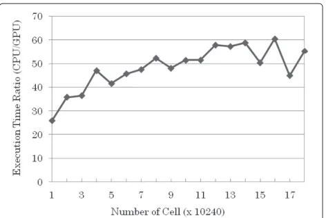
In the experiments, the size of the homogeneous sheet was varied from 10240 (10240× 1) to 1433600 (10240 × 14) cells with 10240-cell increments. The computa-tion time was measured for each increment. Figure 10 shows the CPU and GPU computational time at differ-ent cell array sizes. Results showed that by using the GPU, the computational time can be accelerated 50 times as compared to using a standard CPU.

Discussion

Traditionally, biological function simulation programs have to be manually created from scratch. This is manage-able with small models or simulation experiments but it becomes less practical once model complexity increases. The more complex the model becomes the larger the program becomes and the harder it is to create and main-tain such programs. The Doty model [12] showed that the cost of software development is proportional to the square exponential of the number of computational steps. As seen from Table 4, the number of computational steps increases with the complexity of the model. By using this system, the creation of a simulation program from

Figure 10CPU and GPU execution time ratio of the excitation propagation simulation.

biological models becomes simpler. The system takes input from experts in biological functions through CellML models and mathematical experts through ODE numeri-cal solutions and automatinumeri-cally generates the simulation code. The automatic code generation allows it to deal with large and complex models without the proportional increase in software development cost. This also keeps the software maintenance cost low since the programs are cre-ated with the same structure, regardless of the biological model under study.

The system’s support for multiple programming lan-guages makes it easier for users to test the model in different programming environments and keep the cost of switching from one programming language to a low. Based on the codes generated for the purpose of this paper, science and engineering students typically create a Java simulation code from the C version within four days. The system requires the formatted RelML file to do the first stage of the algorithm and the RelML information can also be used to automatically determine the bound-ary conditions. The RelML information can be extracted automatically from the CellML model file but boundary conditions are not always available. We need a mathemati-cal representation of boundary conditions which are com-patible with declarative description. This can be addressed by the inclusion of PEPML experimental protocol [13] in the system. PEPML is an XML-based language that can describe the initial conditions and procedures of an exper-imental protocol. It describes boundary conditions in a mathematical form and is purely represented in a declar-ative manner, making it easy to combine with the current implementation of our system.

between ODE solving schemes showed that the model can be accurately predicted by the first-order ODE solutions. The use of higher-order numerical solutions has a mini-mal effect on the values of the approximations (Figure 9). The Luo-Rudy model is a set of nonlinear differential equations that use higher order ODE solutions but it can be seen from the Taylor series expansion that equations from the second-order term has little or negligible effect. The structure of the system, where the ODE solver can be easily changed with the appropriate TecML file, allows one to confirm the accuracy of the model simulation such as the case with the Luo-Rudy 1991 model (see Additional file 1).

Although the system is fully implemented, further improvements are still to be added. The generated excita-tion propagaexcita-tion code does not consider the optimizaexcita-tion of the model variables for parallel processing. Therefore, code parallelization is low and may have contributed to slower execution in the GPU environment. Also, the sys-tem can only handle equations with a single term in the left-hand side. Other equation forms will be addressed in future implementations.

Furthermore, simultaneous calculations using differ-ential algebraic equations (DAE) are still not available. Simultaneous equations appear in some models and implicit numerical methods. The handling of implicit methods is available in the inputs but not in the cur-rent implementation of our system. A simultaneous equation library, other ODE numerical solutions library like CVODE, or a linear algebra library like LINPACK could be incorporated into our system. This can be a possibility with our plan to design a library interface description language to handle numerical solution inputs. Future implementations also need to address the need for a declarative design of describing procedural methods. Complex ODE numerical methods like the ones described in the Kinetic Simulation Algorithm Ontology (KiSAO) [14] are difficult or impossible to encode in the current version of TecML. We are in the process of redesigning TecML and the system to incorporate methods that are suitable for the types of problems scientists are addressing with manually-created code, including adaptive methods. This can greatly enhance the usability of the proposed method.

In addition, the system may be integrated with SED-ML. SED-ML allows description of the simulation environ-ment, which includes the name of the numerical method to be used in the simulation. A starting point for inte-gration would be to provide TecML information of a numerical method for the KiSAO entry in SED-ML to allow simulation software to refer to this description. Another point would be to create support for SED-ML files in the code generation system in order to create more complex experiments that use more than one model or

experiments with different simulation methods applied. This will allow users the flexibility of choosing not only the ODE solving methods but also the experiment protocol when generating their simulation codes.

Conclusion

In this paper, we proposed a method to automatically generate executable simulation codes using CellML phys-iological models and ODE numerical solution methods. The generated code describes the time-evolution of the set of differential equations enumerated by the CellML model. The code generation system is composed of a two-stage approach that allows flexible generation of complex sets of equations.

To evaluate the effectiveness of the proposed system, several combinations of physiological cell models and ODE solving schemes were generated. The output of the numerical approximations were in accordance with the published results of the cell models. Results for the Luo-Rudy 1991 simulations also indicated that it only has first-order accuracy. The comparison of execution time for 2D excitation propagation also showed that the use of GPU can accelerate the processing time by 50 times as compared to a CPU.

The code generation system allows executable simula-tion codes to be easily generated from CellML and TecML files. This can be very useful in the field of biological model simulation since it provides the tools to quan-titatively evaluate the mathematical equations in these models.

Additional file

Additional file 1: Appendix.

Competing interests

The authors declare that they have no competing interests.

Author’s contributions

FRP has been involved in the drafting of the manuscript, programming and gathering of experimental data. YY was responsible for programming of the code generator software and gathering data. NS was the main programmer of the code generator. MK was involved in the simulation experiments and data gathering as well as programming. TS, HK and YK acted as consultants for the algorithm and system design. AA has been the main architect of the algorithms and system design and has given the final approval of the version to be published. All authors read and approved the final manuscript.

Acknowledgements

The authors would like to thank the Japan Ministry of Education, Culture, Sports, Science and Technology (MEXT) for the Grant-in-Aid for Scientific Research (Kakenhi) funding.

Author details

1_{Graduate School of Life Sciences, Ritsumeikan University, Shiga, Japan.}

2_{Graduate School of Information Science and Engineering, Ritsumeikan}

University, Shiga, Japan.3_{ASTEM Research Institute of Kyoto, Kyoto, Japan.}

References

1. Cuellar AA, Lloyd CM, Nielsen PF, Bullivant DP, Nickerson DP, Hunter PJ:

An overview of CellML 1.1, a biological model description language.

Simulation2003,79:740–747.

2. Hucka M, Kitano H:The systems biology markup language (SBML): a medium for representation and exchange of biochemical network

models.Bioinformatics2003,19:524–531.

3. Yoshiyuki A, Yasuyuki S, Yoshiyuki K:Specifications of insilicoML 1.0: a

multilevel biophysical model description language.J Biol Sci2008,

58:447–458.

4. Waltemath D, Adams R, Bergmann FT, Hucka M, Kolpakov F, Miller A, Moraru II, Nickerson DP, Sahle S, Snoep JL, Le Novere, N:Reproducible computational biology experiments with SED-ML - the simulation

experiment description markup language.BMC Syst Biol2011,5:198.

5. Fitzhugh R:Impulses and physiological states in theoretical models

of nerve membrane.Biophys J1961,1(6):445–466.

6. Garny A:Cellular Open Source (COR): a public cellml based

environment for modeling biological function.Int J Bifurcation and

Chaos2003,13(12):3579–3590.

7. The CellML Compiler and Code Generator.[http://sourceforge.net/

projects/cellmlcompiler].

8. Luo CH, Rudy Y:A model of the ventricular cardiac action potential,

depolarization, repolarization, and their interaction.Circ Res1991,

68:1501–1526.

9. Matsuoka S, Sarai N, Kuratomi S, Ono K, Noma A:Role of individual ionic current systems in ventricular cells hypothesized by a model study.

Jpn J Physiol2003,53:105–123.

10. Luo CH, Rudy Y:A dynamic model of the cardiac ventricular action potential. I. Simulations of ionic currents and concentration

changes.Circ Res1994,74:1071–1097.

11. Ten Tusscher KH, Panfilov AV:Cell model for efficient simulation of wave propagation in human ventricular tissue under normal and

pathological conditions.Phys Med Biol2006,51:6141–6156.

12. Herd JR, Postak JN, Russell WE, Steward KR:Software cost estimation study: Study results, Final Technical Report, RADC-TR77-220, vol. I. Rockville. Doty Associates: Inc.; 1977.

13. Shimayoshi T, Amano A, Matsuda T:A generic representation format of physiological experimental protocols for computer simulation

using ontology.InEngineering in Medicine and Biology Society, 2007. EMBS

200. 29th Annual International Conference of the IEEE; 2007:382–385.

14. Kinetic Simulation Algorithm Ontology (KiSAO).[www.biomodels.

net/kisao].

doi:10.1186/1751-0473-7-11

Cite this article as:Punzalanet al.:A CellML simulation compiler and code generator using ODE solving schemes.Source Code for Biology and Medicine

20127:11.

Submit your next manuscript to BioMed Central and take full advantage of:

• Convenient online submission

• Thorough peer review

• No space constraints or color figure charges

• Immediate publication on acceptance

• Inclusion in PubMed, CAS, Scopus and Google Scholar • Research which is freely available for redistribution