JIEM, 2017 – 10(2): 352-372 – Online ISSN: 2013-0953 – Print ISSN: 2013-8423 https://doi.org/10.3926/jiem.2158
Determining Decoupling Points in a Supply Chain Networks
Using NSGA II Algorithm
Mina Ebrahimiarjestan1 , Guoxin Wang2
1Department of Industrial Engineering, Kharazmi University, Tehran (Iran) 2School of Mechanical Engineering, Beijing Institute of Technology, Beijing (P.R. China)
[email protected], [email protected]
Received: November 2016
Accepted: January 2017
Abstract:
Purpose: In the model, we used the concepts of Lee and Amaral (2002) and Tang and Chen
(2009) and offer a multi-criteria decision-making model that identify the decoupling points to aim to minimize production costs, minimize the product delivery time to customer and maximize their satisfaction.
Design/methodology/approach: we encounter with a triple-objective model that
meta-heuristic method (NSGA II) is used to solve the model and to identify the Pareto optimal points. The max (min) method was used.
Findings: Our results of using NSGA II to find Pareto optimal solutions demonstrate good
performance of NSGA II to extract Pareto solutions in proposed model that considers determining of decoupling point in a supply network.
Originality/value: So far, several approaches to model the future have been proposed, of
Keywords: industrial systems, analysis points, pareto optimal points, multi-criteria decision, meta-heuristic algorithm
1. Introduction
2. Literature Review
2.1. Separation Point
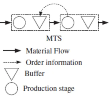
Decoupling points in a supply chain network are areas that break down the production line to lean manufacturing system and agile manufacturing system. Lean manufacturing is based on the strategy of make to stock (MTS). In MTS, products are stored in the warehouse until they create demand for products. Then the products are delivered from the warehouse to the customer, and the good delivery to the customer is as a pulse for the last station on the assembly line. There is a pulse to produce the station from beginning the process in each station to the output from the previous station. In lean manufacturing, it is clear that the goods or services that delivered to the customer are based on the standard characteristics, and the specific feature of the customer is not considered. The advantage of this strategy is that the product delivery time to the customer is at its minimum level. Such a mechanism is shown in Figure 1.
Figure 1. Make to storage (lean manufacturing)
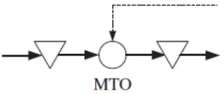
Figure 2. make to order (agile technology)
According to the above description, each strategy has advantages and disadvantages. So a good strategy can use the advantages of both. The concept is expressed using decoupling points in a supply chain network. So a supply network can be decomposed into two parts, the upstream and downstream sectors. The upstream section includes manufacturing operations from the beginning of the production process to decoupling points and downstream is from break point until the end of production lines. MTS and MTO strategies are used in the upstream and downstream sectors respectively. In literature, MTS and MTO are presented with the other titles like compressive and tensile strategies.
To identify decoupling points, three important aspects should be considered:
1. Minimization of the production cost
2. Minimization of the delivery time to the customer
3. Maximization of the customer satisfaction.
So we faced with a multi-objective problem.
Figure 3. The supply product chain (Sun et al., 2008)
In Figure 5, the nodes show products. Here, the required raw materials are shown by Pi and semi-finished products during the manufacturing process and the final product will are shown by Ai. In the model, we used the concepts of Lee and Amaral (2002) and Tang and Chen (2009) and offer a multi-criteria decision-making model that identify the decoupling points to aim to minimize production costs, minimize the product delivery time to customer and maximize their satisfaction.
The way to solve the problem and choosing the MTO and MTS is a meta-heuristic Algorithm that chooses only the optimal points of Pareto. Finally, with delivery of these points to the management, he is responsible to make the final decision from these points.
Agarwal, Shankar and Tiwari (2006) have presented a network analysis process-based framework in order to modelling the performance measurement of three strategies in supply chain (Lean, Agile, Lean/Agile). The main aim of this studies was the performance evaluation and the selection of most appropriate strategy in order to enhancing the supply chain performance. Additionally, cost, quality, service level and waiting time were the four major criteria in supply chain factor analysis. These investigations showed the lean/agile is the most appropriate strategy for improving supply chain performance. This results also shows the tendency of managers in order to runs policies for combining the lean and agile approaches in supply chain (Agarwal et al., 2006).
Krishnamorti and Yauch (2007) have studied the implementing capability of lean/agile fabrication strategy in manufacturing company which has several business units. They results showed that the agile and lean fabrication are the supportive strategies and manufacturing companies can use these strategies, simultaneously. Moreover, a theoretical infrastructure for lean/agile model in which lean and agile strategies are acting in different part of the company and are separated by a breakpoint have presented. The proposed infrastructure is made of decentralized organizational structure with small and medium-sized for agility, and the centralized organizational structure with large and medium-sized for leanness (Krishnamurthy & Yauch, 2007).
Regarding to the discussed features, lean supply chain cannot meet the customer needs, quickly. Therefore, lean/agile supply chain which combines the benefits of lean and agile supply chain have been recommended. In fact, lean/agile supply chain with combining lean and agile strategies provides rapid response to changing demands of upstream and downstream companies with maintaining and consolidating its own position in the supply chain Cao and Zhang (2011). Based on the major goal of the supply chain, customer satisfaction, Naim and Gosling (2011), quoting Johnson, have defined four criterion as a main criterion for comparing lean and agile supply chain. These criteria are services, quality, cost and waiting time which agility and leanness value of supply chain are depend on the size of them (Gosling, Purvis, L., Naim, 2010).
Perez, Castro, Simons and Gimenez (2010) have analyzed the performance and features of Catalan meat supply chain with the aim of whether those responsible for lean supply chain is used in the industry. In this regard, a conceptual model have used as an evaluation tool. (Perez et al., 2010).
Based on a review of the ‘leagile’ literature, Nieuwenhuis and Katsifou (2015) shows that a new understanding of the factors that determine the ‘decoupling point’ between lean and agile processes can be used in order to bring about a radical shift in economies of scale in car production. In this way, lower volume production becomes feasible thereby reducing the need for overproduction and enabling a move towards more sustainable car production and hence consumption. By way of illustration, you should consider how Morgan Motor Company implement such an approach in practice (Nieuwenhuis & Katsifou, 2015).
3. Modeling of the Problem
3.1. Decision Variable
Decision variable in this model is to produce every product with the strategy of MTO or MTS, hence the decision variables is considered as Oi in follows:
(1)
3.2. Delivery Time
The arcs of the network between every of two nodes indicates the processes to convert the two products in both nodes is done. These activities include manufacturing processes and assembly products. Each arc includes a time (uptime) and so the delivery time of product is as long as the root node to the end node, and so is equal to the critical time of the network. So if activities on the network were shown with MTO and MTS, as mentioned above, the MTS activities have the least amount of possible delivery time and therefore the time of the activities in the delivery to client is considered negligible and zero. Also, for the activities that are produced as MTO, The total time of product in different workstations is the time of delivery to the customer. So to extract the time of delivery to the customer from the network, all the directions from the beginning node to the end one are consider. Time activities of MTO on the every track are sum up is that the delivery time of goods from the track to the customer. The longest of these times is the delivery time of goods to the customer. So delivery time of goods to customers T can be obtained from the following equation:
(2)
3.3. The Fee Structure
In problem modeling, regarding that the decision variable means every production activity to be produced by MTS or MTO, we determine the cost structure considering this variable in which there is the meaningful effect in present of MTS and MTO. In other words, the only costs are considered when MTS and MTO are chosen. For examples, the cost that is common in both strategies is neglected, and the only cost that differs in MTS and MTO i considered. In MTS strategy activities, production is based on prediction and the product is provided in standard terms, not the ordered and then there is no need to modification of production structure and product design. Noted, in MTS the products stored in the warehouse, the cost of storage is one of the main components of cost, and as we know in MTO because the product is produced strictly according to demand, there is no cost like this. Another cost structures that differ between MTO and MTS is the cost preparation. The one for MTO is relatively high because these costs are considered for each of the products that are produced. In MTS, the products are produced as batch production, so these costs are limited only to the category of the production.
At MTO also, there a cost of customizing that can be considered as costs of production adjustment and design. In this study, we assume that the order is constant that is shown by D in the planning horizon. To obtain the demand for intermediate products, we use the bills of materials (BOM) and perquisite relationships of the network. The materials bill is shown by BOM matrix in which BOM (i, j) represents the number of products from i that is required to produce a unit of product of j. So if the demand for product j is shown by Dj, the product demands for i is obtained by the following equation:
(4)
We assume a constant rate of production of each product. Also in the modeling notations we have:
Si: preparation cost for product i
Hi: The cost of maintenance for each unit of product j in a year
ui: production rate
pi: demand rate
(5)
On the other hand, if we consider the activity as MTO, the cost of preparing a must for all demands will be addressed in other words the cost of preparation. As well as the cost of customization for all applications also assume that if the price customizing of the product i is CSi, the cost will be equal to customizing the product i. So for product i that the MTO is produced, the cost will be as follows:
(6)
3.4. Customer Satisfaction
As noted, one of the goals of our model is to maximize customer satisfaction. Maximizing customer satisfaction ensures future demand of products and company profit in development outlook. In this model, we assume that if the product to be produced as standard (strategy MST), customer satisfaction is the product SFi and if the product is customized production (strategy MTO) customer satisfaction is CFi.
CFi is larger than SFi. CFi and SFi values can be calculated using value analysis and qualitative studies such as analysis factor; however, in this case, we assume that this information is already known. So the customer satisfaction of product i can be expressed as follows.
3.5. Prerequisites Restrictions
Prerequisite is defined because if product i was produced with MTO manufacturing strategy, all products that are related to this product, in another word the product i is their prerequisite product before they need to be produced with MTO strategy. This restriction has, in fact, the concept of decomposition point that divides production line and supply chain network into two parts of upstream and downstream. Hence, these restrictions should also be added to the model.
(7)
4. The Proposed Solution Method
4.1. NSGA II Algorithm
Non-Dominated Sorting Genetic Algorithm (NSGA-II), a popularly used algorithm proposed by Deb, Pratap, Agarwal and Meyarivan (2002) offers a great approach to deal with multi-objective optimization problem. This algorithm has some improvement over the original one (Srinivas & Deb, 1995). In this section, we describe this algorithm briefly. Details can be found in Deb (2001). In NSGA-II, firstly the offspring population Qt is formed from the parent population Pt. The combination of two populations is
Rt of size 2N. Then a non-dominated sorting classifies the entire population Rt. This process will allow a global non-domination check among the offspring and parent solutions (Deb, 2001). Two most important concepts in NSGA-II are a fast non-dominated sorting of the solutions population and a crowding distance calculation.
Crowding distance calculation: This procedure is used as an estimation of solutions near a particular
Fast non-dominated sorting: Here we form a non-dominated set of solution. The first solution from the set is kept in a set P. Then, each subsequent solution is compared with all members of the set P. If the solution q is dominated by p, then solution q is removed from P. Thus, these dominated solutions get eliminated from P. Otherwise, if any member of P dominates the solution p, p is disregarded. The solution p entered in P if it is not dominated by any member of P. After that all check is done, the solution set P, considered as a non-dominated set. The procedure is as follow (Deb, 2001):
Fast- non-dominated-sort (P)
For each pP Sp = Ø
np= 0
For each qP
if (p < q) then
Sp = SpU {q} else (q < p) then
np= np + 1 if np= 0 then Prank = 1 f1 = f1U {p}
i = 1 while fi ≠ Ø
Q = Ø
for each pfi for each qsp
nq= nq – 1 if nq= 0 then qrank = i +1 Q = Q U {q} i = i +1
Fi = Q
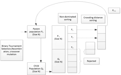
tournament selection, recombination, and mutation operators are executed to generate the population of the following generation, Q0, of size N. The procedure (Figure 4), for the remaining generation (for t ≥ 1) is as follows (AL-Fayyaz, 2004):
Step 1. First a combined population (parent and offspring) of size 2N, Rt = Pt UQt is formed, which is sorted according to a fast non-domination procedure. This step results in different non-dominated fronts
F1, F2, etc.
Figure 4. Graphical diagram of NSGA-II Algorithm (Deb, 2001)
Step 2. The new parent population Pt+1 is formed by adding solutions from the first front F1 and continuing till the size exceeds N;
Step3. The solutions of the last accepted front are sorted according to a crowded comparison criterion (to maintain diversity in the population, this criterion is used which prefers a point that is located in a region with lesser number of points) and a total of N points are picked;
is important to mention here that the non-dominated sorting in step 1 and filling up population Pt+1 can be performed together. In each time a non-dominated front is found, its size can be checked whether it can be included in the new population. If not, then no more sorting is needed. This will reduce the run time of the algorithm.
4.2. Numerical Examples
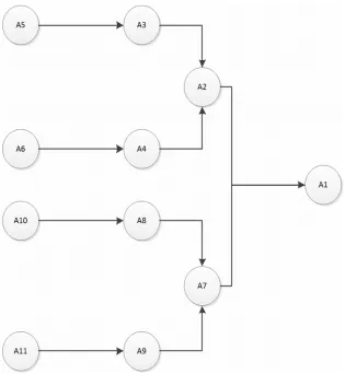
Consider following supply chain network shown in Figure 5:
Figure 5. supply chain network example
We use a string that contains 11 bit to represent a solution of this model. Each bit takes value 0, if corresponding operation be MTO and 1 otherwise. For example the representation D1 shows the solution that operations A1, A2 and A7 are MTO operation and other operations are MTS; in other words operations A2 and A7 act as decoupling points:
This network has parameters as below:
CS = [10 9 7 8 6 6 9 8 7 8 9];
T = [6 6 6 6 1 8 10 4 10 4 9];
S = [2 2 1 1 2 3 4 3 1 4 4];
H = [0.77 0.04 0.37 0.70 0.72 0.22 0.27 0.67 0.47 0.62 0.24];
sf = [0.18 0.83 0.76 0.93 0.11 0.18 0.1 0.49 0.19 0.89 0.1];
cf = [0.35 1.66 1.53 1.87 0.21 0.36 0.2 0.97 0.38 1.79 0.19];
p = [5 8 9 6 6 7 6 8 10 8 5];
d = 69;
u = [4.0 6.4 7.2 4.8 4.8 5.6 4.8 6.4 8.0 6.4 4.0];
Here, element i of each vector, corresponds to related vector parameter of operation i.
Also, each solution like D1 is labeled with a matrix that shows the value of operations in the solution corresponding to all routs that originate from the final product (in this example A1) and terminate to network leaves (here A5, A6, A10 and A11). This matrix is useful when we want to compute final product delivery time and use crossover operation in NSGA II to generate new solutions. In the network in Figure 5, there are four routs that are A1-A2-A3-A5, A1-A2-A4-A6, A1-A7-A8-A10, and A1-A7-A9-A1. In the labeled matrix for each rout, we have a row that has n elements (n is equal to the number of all operations). The element of labeled matrix is defined as follow:
(8)
For example labeled matrix of solution D1 is as follow:
(9)
As mentioned in section 3, each operation has a time (the vector T shows time of each operation) and if that operation is considered as MTO, affects delivery time in constraint (3) and (4). Now we can easily compute final product delivery time as follow:
(11)
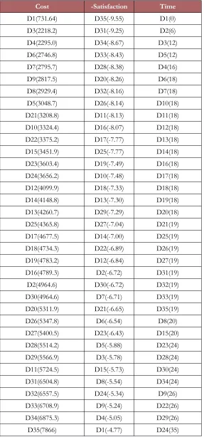
In the network of Figure 4, there are 35 combinations of MTO and MTS operations; therefore we have 35 solutions which must be considered. Matrix D shows all 35 representations.
In Table 1, which Di corresponds to solution i, the objective functions regarding each solution are shown in the descending order as we have expected there is some conflict between model objectives For example, while solution D1 has maximum utility considering cost, it has minimum customer satisfaction. For above example we have all Pareto optimal solutions as below:
Pareto Optimal Solutions = [D1 D2 D3 D5 D6 D7 D10 D16 D17 D20 D25 D28 D31 D35];
• Adjust solution D:
◦ When making a new solution, if an operation is considered as MTO, all operations that
originated from that operation and terminated at final operation are also considered MTO.
◦ When making a new solution, if an operation is considered as MTS, all operations that originated from that operation and terminated at final leaves also is considered MTS.
• Initialization:
◦ Generate K initial solution For i = 1 to k
-select p1 randomly between 0 and 1 -select p2 randomly between 0 and 1 -if p1 < 0.5
-j 1 = random number between 1 to 6 -Di ( j1) = 1;
-adjust Di -if p2 < 0.5
-j 2=random number between 7 to 11 -Di ( j2) = 1;
-adjust Di • Crossover:
-assume Di is corresponding to parent 1 with labeled matrix Si, and Dj is corresponding to parent 2 with labeled matrix Sj
-select one row of Si randomly -select one row of Sj randomly
-exchange two random rows, between Si and Sj -generate two new solutions based on new Si and Sj • Mutation:
-select q1 randomly between 0 and 1 -if q1 < 0.1
-Select one operation randomly and changed its corresponding value In the current solution. For example, if its value is 1, change it to 0 and if Its value is 0 change it to 1.
Cost -Satisfaction Time
D1(731.64) D35(-9.55) D1(0)
D3(2218.2) D31(-9.25) D2(6)
D4(2295.0) D34(-8.67) D3(12)
D6(2746.8) D33(-8.43) D5(12)
D7(2795.7) D28(-8.38) D4(16)
D9(2817.5) D20(-8.26) D6(18)
D8(2929.4) D32(-8.16) D7(18)
D5(3048.7) D26(-8.14) D10(18)
D21(3208.8) D11(-8.13) D11(18)
D10(3324.4) D16(-8.07) D12(18)
D22(3375.2) D17(-7.77) D13(18)
D15(3451.9) D25(-7.77) D14(18)
D23(3603.4) D19(-7.49) D16(18)
D24(3656.2) D10(-7.48) D17(18)
D12(4099.9) D18(-7.33) D18(18)
D14(4148.8) D13(-7.30) D19(18)
D13(4260.7) D29(-7.29) D20(18)
D25(4365.8) D27(-7.04) D21(19)
D17(4677.5) D14(-7.00) D25(19)
D18(4734.3) D22(-6.89) D26(19)
D19(4783.2) D12(-6.84) D27(19)
D16(4789.3) D2(-6.72) D31(19)
D2(4964.6) D30(-6.72) D32(19)
D30(4964.6) D7(-6.71) D33(19)
D20(5311.9) D21(-6.65) D35(19)
D26(5347.8) D6(-6.54) D8(20)
D27(5400.5) D23(-6.43) D15(20)
D28(5514.2) D5(-5.88) D23(24)
D29(5566.9) D3(-5.78) D28(24)
D11(5724.5) D15(-5.73) D30(24)
D31(6504.8) D8(-5.54) D34(24)
D32(6557.5) D24(-5.34) D9(26)
D33(6708.9) D9(-5.24) D22(26)
D34(6875.3) D4(-5.05) D29(26)
D35(7866) D1(-4.77) D24(35)
In this example we set initial size of population equal to 8, therefore in each iteration we must consider a population of size 16. Using this algorithm we have final Pareto solutions as follow:
D16, D5, D1, D28, D35, D6, D17, D25, D31;
We now face with problem of choosing solution among Pareto optimal solutions. In fact the answer is based on managerial consideration. Nonetheless we can find some suggestions in literature to cope with this problem. For example we can use following methods:
• Max-min:
(12)
• Normalized membership ranking:
(13)
(14)
In this way the solution with higher μk has greater rank.
5. Conclusion and Future Research Directions
Meta-heuristic methods need to be examined for performance testing. But there is an important issue here is how it can be argued that the proposed method, this is an effective method. To answer this question it is necessary to use several methods to assess the suitability of the results they achieved an overall result (Arjestan, 2016)
composed of MTS operations that use standard features and refers to lean production systems and the second part is composed of MTO operations that adjust production to meet specific customer orders. Therefore, efficient determination of decoupling point has found great interest in production concepts. In this paper, we presented a new model to address this problem as an MODM problem. The proposed model here minimizes production cost, delivery time and maximizes customer satisfaction as its objectives and considering operations as MTO or MTS as binary decision variables.
NSGA II is a known algorithm to address MODM problem when decision space is discrete. In this study, we used NSGA II algorithm to find some non-dominated solutions of the problem and present some suggestion to select final solution through Pareto optimal solutions. However, we remember again that choosing between Pareto optimal solutions depends on senior manager decisions and considerations.
Our results of using NSGA II to find Pareto optimal solutions demonstrate good performance of NSGA II to extract Pareto solutions in proposed model that considers determining of decoupling point in a supply network.
In this study, we assume the demand of the product is deterministic and fixed. There is a great area to address decoupling point determination problem with another demand trend such as stochastic demand, demand with fixed batch size, demand reached in fixed interval and so on, that we suggest them for future research. Also we can solve such MODM problem with other methods such as goal programming,
ε-constraint, etc., by considering real world application problems.
References
Aitken, J., (2000) Agility and Leanness – A Successful and Complimentary Partnership in the Lighting Industry. Proceedings LRN 2000 Conference. 1-7.
Agarwal, A., Shankar, R., & Tiwari, M.K. (2006). Modeling the metrics of lean, agile and leagile supply chain: An ANP-based approach. European J. of Operational Research, 173, 211-225.
https://doi.org/10.1016/j.ejor.2004.12.005
Agarwal, A., Shankar, R., & Tiwari, M.K. (2007). Modeling agility of supply chain. Journal of Industrial Marketing Management, 36, 443-457. https://doi.org/10.1016/j.indmarman.2005.12.004
Arjestan, M. (2016). Efficient Optimization of Multi-Objective Redundancy Allocation Problems in Series-Parallel Systems. Decision Science Letters, 6(3), 307-322. https://doi.org/10.5267/j.dsl.2016.11.004
Cao, M., Zhang, Q. (2011). Supply chain collaboration: Impact on collaborative advantage and firm performance. Journal of Operations Management, 29(3), 163-180. https://doi.org/10.1016/j.jom.2010.12.008
Christopher, M., (2000). The Agile Supply Chain: Competing in Volatile Markets. Ind. Mark. Man., 29(1), 37-44. https://doi.org/10.1016/S0019-8501(99)00110-8
Christopher, M., & Towill, D. (2001). An Integrated Model for the Design of Agile Supply Chaines.
International Journal of Physical Distribution & Logistics Management, 31(4).
https://doi.org/10.1108/09600030110394914
Deb, K. (2001). Multi-objective Optimization Using Evolutionary Algorithms. Chichester, U.K.: Wiley.
Deb, K., Pratap, A., Agarwal, S., & Meyarivan, T.A.M.T. (2002). A fast and elitist multi-objective genetic algorithm: NSGA-II. Evolutionary Computation, IEEE Transactions, 6(2), 182-197.
https://doi.org/10.1109/4235.996017
DeGroote, S.E., & Marx, T.G. (2013). The impact of IT on supply chain agility and firm performance: An empirical investigation. International Journal of Information Management, 33, 909-916.
https://doi.org/10.1016/j.ijinfomgt.2013.09.001
Gosling, J., Purvis, L., Naim, M. (2010). Supply chain flexibility as a determinant of supplier selection.
International Journal of Production Economics, 128(1,: 11-21.
Krishnamurthy, R., & Yauch, C.A. (2007). Leagile manufacturing: A proposed corporate infrastructure,
Int. J. Of Operations and Production Management, 27(6), 588-604. https://doi.org/10.1108/01443570710750277
Lee, H.L., & Amaral, J. (2002). Continuous and sustainable improvement through supply chain performance management. Standford Global Supply Chain Management Forum SGSCMF. 1-14.
Naim, M.M., & Gosling, J. (2011). On leanness, agility and leagile supply chains. International Journal of Production Economics, 131(1), 342-354. http://doi.org/10.1016/j.ijpe.2010.04.045
Nieuwenhuis, P., & Katsifou, E. (2015). More sustainable automotive production through understanding decoupling points in leagile manufacturing. Journal of Cleaner Production, 95, 232-241.
https://doi.org/10.1016/j.jclepro.2015.02.084
Perez, C., Castro, R., Simons, D., & Gimenez, G. (2010) Development of lean supply chains: a case study of the Catalan pork sector. Supply Chain Management: An International Journal, 15(1), 55-68.
https://doi.org/10.1108/13598541011018120
Srinivas, N., & Deb, K. (1995). Multi-objective function optimization using non-dominated sorting genetic algorithms. Evolutionary computation, 2(3), 221-248. https://doi.org/10.1162/evco.1994.2.3.221
Sun, X.Y., Ji, P., Sun, L.Y., & Wang, Y.L. (2008). Positioning multiple decoupling points in a supply network. International Journal of Production Economics, 113(2), 943-956.
https://doi.org/10.1016/j.ijpe.2007.11.012
Tang, D., & Chen, J. (2009). Identification of postponement point in service delivery process: A description model. Service Systems and Service Management, ICSSSM'09, 6th International Conference on IEEE.
335-339.
Journal of Industrial Engineering and Management, 2017 (www.jiem.org)
Article’s contents are provided on an Attribution-Non Commercial 3.0 Creative commons license. Readers are allowed to copy, distribute and communicate article’s contents, provided the author’s and Journal of Industrial Engineering and Management’s