VOLUME 37, ARTICLE 47, PAGES 1515
,
1548
PUBLISHED 23 NOVEMBER 2017
http://www.demographic-research.org/Volumes/Vol37/47/ DOI: 10.4054/DemRes.2017.37.47
Research Article
Decomposing American immobility:
Compositional and rate components of
interstate, intrastate, and intracounty
migration and mobility decline
Thomas B. Foster
© 2017 Thomas B. Foster.
This open-access work is published under the terms of the Creative Commons Attribution 3.0 Germany (CC BY 3.0 DE), which permits use, reproduction, and distribution in any medium, provided the original author(s) and source are given credit.
1 Introduction 1516
2 Background and theory 1517
2.1 The determinants of mobility 1517
2.2 Population composition and aggregate mobility and migration 1518
2.3 Spatial perspectives on American immobility 1520
3 Data and methods 1521
3.1 The Oaxaca–Blinder decomposition method 1521
3.2 Measuring annual migration and mobility in the CPS 1523 3.3 Individual-level predictors of mobility and migration 1524
4 Results 1525
4.1 Stage one results: Predicting individual mobility in 1982 and 2015 1528 4.2 Stage two results: Compositional components of migration and
mobility decline between 1982 and 2015 1530
4.3 The impact of the Great Recession and foreclosure crisis 1533 4.4 Rate components of mobility and migration decline: Age, race, and
geography 1535
5 Conclusion 1540
6 Acknowledgments 1542
Decomposing American immobility:
Compositional and rate components of interstate, intrastate,
and intracounty migration and mobility decline
Thomas B. Foster1
Abstract
BACKGROUND
American migration rates have declined by nearly half since the mid-20th century, but it is not clear why. While the emerging literature on the topic stresses the salience of shifts in the composition of the American population, estimates of the contribution of population aging, increasing diversity, rising homeownership, and other shifts vary widely. Furthermore, it is unclear whether and how compositional shifts differ in their effects on migration over different geographic scales.
OBJECTIVE
To gauge the contribution of compositional shifts to concomitant declines in migration over various distances, while allowing for group variations in the rates at which declines occur.
METHODS
Drawing on individual-level IPUMS Current Population Survey data from 1982 to 2015, I use the Oaxaca–Blinder method to decompose declines in interstate migration, intrastate migration, and intracounty mobility.
RESULTS
Between a quarter and a third of declines since 1982 are attributable to aging and increasing diversity. Changing ethnoracial composition exerts a stronger influence on interstate migration, while aging has a stronger effect on local mobility. Results also reveal more dramatic declines among non-Latino Whites and those under age 35, as well as a marked delay and decline in peak mobility rates with each successive birth cohort.
CONCLUSIONS
Results point to social and economic shifts as the key drivers of American immobility, and the need for reorientation within the emerging literature. Future research should
investigate the causes of group-specific rates of decline and focus on local mobility, where declines are most concentrated and where rising immobility is most problematic.
1. Introduction
The typical American is now half as likely to have moved in the past year as their counterpart in 1950 (Cooke 2011; Fischer 2002; Molloy, Smith, and Wozniak 2017). This is true for both long-distance migration and local mobility, as well as for Americans of nearly all sociodemographic or socioeconomic statuses. Despite the universality of this trend, little work has considered the causes and consequences of immobility in the United States. Though they remain unclear, the forces driving American immobility must be “deep and pervasive” (Fischer 2002: 193) and “affect a large fraction of the workforce and broad swaths of the economy” (Molloy, Smith, and Wozniak 2017: 23).
Most commonly, explanations of migration and mobility decline point to substantial changes in the composition of the American population since the mid-20th
century in favor of typically less mobile groups. Population aging, increasing racial/ethnic diversity, post-1965 era immigration, increasing homeownership rates, the growing prevalence of dual-earner households, changing family structures, and the rise in long-distance and telecommuting are all included in this discussion. But the contribution of any of these shifts is difficult to pin down with certainty. Consider the role of population aging, which is arguably the most commonly cited cause of migration and mobility decline. Estimates of the contribution of population aging to overall declines vary greatly and are to some degree dependent upon the distances or boundaries over which movement is measured. On the one hand, Molloy, Smith, and Wozniak (2014: 1) find that while population aging and rising homeownership rates explain about half of all local, intracounty mobility decline, effectively none of the decline in interstate mobility is attributable to these factors. On the other hand, Karahan and Rhee (2014) argue that at least half of all the slowdown in interstate mobility is attributable to population aging, particularly through the calming effect that middle-aged workers have on the job transition decisions of younger workers.
and further limit access to quality neighborhoods (Crowder and South 2005; Massey 1996; South and Crowder 1997). If population aging or rising homeownership drive declines, for example, then these negative impacts and the need for policy intervention may be overstated. However, if rising costs of or diminishing returns to mobility are to blame, then immobility is much more problematic.
I use data from the Current Population Survey to clarify both the role of compositional population shifts in observed mobility declines and how that role changes (if at all) over different distances or boundaries by decomposing changes in annual interstate, intrastate, and intracounty movement between 1982 and 2015. I identify the proportion of overall declines attributable to shifts in population age structure, wages, homeownership rates, dual-earner household shares, family structure, and racial/ethnic composition. In addition to gauging these compositional effects, the Oaxaca–Blinder decomposition method I utilize also identifies group-specific changes in the rates at which migration and mobility decline occur. Results show substantial variations in the rates of migration and mobility decline by race/ethnicity and age group that have not received due attention in the emerging literature, and which contribute to our nascent understanding of the underlying causes and consequences of the American mobility decline.
2. Background and theory
2.1 The determinants of mobility
socioeconomic status because those with more economic resources, higher levels of education, and higher levels of human capital are better situated to overcome the costs associated with movement. The costs of mobility are typically higher for families than for individuals, and therefore single individuals are typically more mobile. Households with two earners have to find two new jobs at the destination instead of just one; households with children must make difficult decisions about school districts and funding; and as family size increases, economic and social costs of mobility increase. Finally, mobility and migration rates tend to be higher among the young and decline with age, because the young have a longer period of time over which the costs associated with mobility can be recouped (Long 1988).
2.2 Population composition and aggregate mobility and migration
Any aggregate shift in the composition of the US population produces an associated shift in the cost calculus among potential movers (Long 1988). Population aging, for example, means that the typical mover has less time to recoup costs. Rising homeownership and dual-earner shares mean that the typical move is more costly and difficult than before. Stagnating wages and the hollowing-out of the middle class means that the typical mover has fewer resources to leverage against the costs of migration and mobility. And so on.
The aggregate population shifts witnessed in the past five decades should place upward pressure on the costs associated with mobility for the typical American, while at the same time reducing the pool of resources for mitigating, and time available for recouping, any losses. The median age in the United States increased from 30.2 to 37.2 between 1950 and 2010, due in large part to aging baby boomers and declining fertility in subsequent generations (Hobbs and Stoops 2002). Despite population aging, the American population continues to grow due to continued post-1965-era immigration from Latin America and Southeast Asia (Frey 2015). Because younger and native non-Latino White populations tend to be more mobile, population aging among native whites, immigration, and increasing racial and ethnic diversity should contribute to aggregate migration and mobility decline.
mobility since 1980, it accounts for effectively none of the slowdown in interstate migration over the same time period. Contrary to this report, however, Karahan and Rhee (2014) demonstrate that population aging plays a much larger but more subtle role in interstate migration decline than Molloy and colleagues allow. They find that the aging of the labor force and the growing share of middle-aged workers exert a calming equilibrium effect on the migration decisions of younger workers. In total, they find that about 50% of the observed decline in interstate migration since the mid-1980s can be attributed to population aging and its “spillover” effects on younger workers (Karahan and Rhee 2014). As such, it remains unclear how population aging and other compositional shifts, which some deem worthy of the moniker “Third Demographic Transition” (Coleman 2006; Lichter 2013), have influenced mobility and migration rates in the United States.
Like population aging and increasing ethnoracial diversity, shifts in the characteristics and structure of the typical household over time may influence aggregate rates. The past five decades have seen rising divorce rates, as well as delayed and reduced rates of marriage and fertility (Lesthaeghe and Neidert 2006). Key life-cycle transitions such as marriage, divorce, and childrearing often necessitate mobility for at least some individuals in the family unit. Increasing divorce rates may place upward pressure on mobility and migration, but declining and delayed marriage and fertility may contribute to mobility slowdowns. Recent decades have also seen rising rates of homeownership and the increasing prevalence of dual-earner households (Molloy, Smith, and Wozniak 2011). Because of the complexities inherent in selling and buying a home, and because it is more difficult to find work in a new labor market for two earners than for one, increasing homeownership and dual-earner shares should place downward pressure on movement.
It also is possible that this bifurcation in labor market structures has made labor markets in the United States more similar over time, reducing the incentive for workers to migrate in search of new opportunities elsewhere (Kaplan and Schulhofer-Wohl 2012). Economic shifts since 1970, therefore, place downward pressure on migration and mobility, as Americans increasingly lack the economic means and incentives to move.
2.3 Spatial perspectives on American immobility
Unlike other demographic processes, migration and mobility are inherently spatial (Mueser 1989; Rogers et al. 2002; Rogers and Sweeney 1998). The pushes, pulls, and intervening costs (Lee 1966) navigated by individuals and families are etched in space, so systematic changes in that space, whether produced by changes in the flow of capital (e.g., Harvey 2010) or by prior population or labor migration, influence movement through it. The emerging literature, however, has largely neglected the role of space in rising immobility. Deviating from this general rule and using a novel modeling approach, Kaplan and Schulhofer-Wohl (2012) show that interstate mobility decline is a function of declining geographic specificity in labor market industrial structures. While others have speculated that interstate migration decline since the 1970s may simply reflect the slowing of the Great Migration (and the regional equilibration of its attendant socioeconomic pushes and pulls) of Southerners to metropolitan destinations in the Midwest, Northeast, and West (Molloy, Smith, and Wozniak 2011), this hypothesis has not been tested rigorously.
The lack of attention lent to spatial structure in the mobility and migration decline literature may contribute to incongruity in reported findings. Indeed, assessments of the contribution of compositional shifts differ, in part, depending on whether and how the role of geographic distance as an intervening cost is considered. Individual decisions to migrate over long distances are usually based on a different set of pushes and pulls than decisions surrounding local mobility (Greenwood 1975, 1985; Long 1988; White and Lindstrom 2006). Long-distance moves are typically undertaken for economic or job-related reasons, such as to find work or relocate to take advantage of regional wage differentials. Residential mobility, however, is usually connected to life-cycle and household changes, such as marriage or separation, child-rearing and schooling, or the transition from renting to owning a home.
migration between states, while life cycle and household shifts will prove more influential for short-distance mobility within counties.
3. Data and methods
3.1 The Oaxaca–Blinder decomposition method
The central goal in this paper is to understand the contribution of population composition shifts to declining interstate, intrastate, and intracounty migration and mobility in the United States. Generally speaking, decomposition methods facilitate this sort of inquiry by posing a counterfactual scenario in which outcomes for one group are predicted as a function of the constituent characteristics of a second group, and vice versa, such that group differences in outcomes for those two groups can be attributed to differences in constituent characteristics. For example, fertility rates in two populations can be decomposed into portions attributable to differences in the age structure of the two populations by applying each population’s age structure to the other’s age-specific fertility rates (e.g., Vaupel and Canudas-Romo 2002).
Oaxaca (1973) and Blinder (1973) provide a parametric generalization of this traditional decomposition framework to model aggregate outcomes for two groups as a function of individual-level characteristics, effectively decomposing macro-level differences into portions attributable to observed and unobserved differences at the micro level. For example, the Oaxaca–Blinder method is often used to decompose the gender wage gap into portions attributable to observed differences in human capital or productivity and to unobserved discrimination in the labor market (Jann 2008). Results also allow the posing of counterfactual scenarios, such as women’s expected wages assuming they saw the same returns to human capital as men, and vice versa. While not useful for establishing causal relationships, these decomposition methods help identify more broadly the likely source of difference in outcomes for two groups and, therefore, directions for future research (Fortin, Lemieux, and Firpo 2010).
logistic models is the area under the receiver operating characteristic curve (or AUC of the ROC). This statistic is preferable to a simple calculation of the percentage of observations correctly predicted because, while the latter is sensitive to the predicted probability threshold chosen for discerning predicted outcomes, the former considers the entire range of potential thresholds from 0 to 1. Intuitively, this area represents the probability that the model correctly orders two randomly chosen individual observations (one a true positive and one a true negative) by assigning a higher predicted probability to the true positive observation. Logistic regression models perform well as gauged by AUC of the ROC and improve substantially on random chance (which would correctly order observations with probability 0.5): AUC ROC statistics for models of interstate, intrastate, and intracounty migration in 1982 are 0.739, 0.697, and 0.737, respectively; corresponding statistics for models of migration in 2015 are 0.734, 0.694, and 0.736, respectively.
Though developed to decompose differences in continuous outcomes, the Oaxaca– Blinder method has been extended to accommodate categorical and other limited outcomes, such as the binary migration/mobility outcome modeled here (Jann 2008). While the logit or probit specification is preferred to the LPM for this outcome, I present results for the LPM here because it eases the interpretation of decomposition coefficients. The main problem with the LPM for binary outcomes is the assumption of homoscedasticity. This assumption is not met in the data, resulting in biased standard errors. However, because the emphasis here is not on statistical inference and hypothesis testing (which are heavily dependent on the correct estimate of SEs), but on (changes in) parameter estimates between two points in time, I opt for the familiar and easily interpretable LPM. Nevertheless, I did compare decomposition results from the LPM to those for logit and probit specifications in supplemental analyses. Broadly speaking, results are robust to the specification of the first-stage model. Interested readers may consult accompanying data and code to compare LPM, logit, and probit results.
The decomposition proceeds in two stages. For the first stage of the decomposition (Jann 2008), consider two linear probability models of individual-level interstate, intrastate, or intracounty movement as a function of individual characteristics at timest
andt+1:
= + ,
and
The second-stage of the decomposition is, therefore,
− = ( − ) + − + ( − ) − .
In the second-stage equation, the first of the three terms on the right-hand side is an estimate of the effect of changing population composition on the overall change in migration or mobility rates based on timetparameter estimates. The second term is an estimate of the effect of changing parameter estimates on the overall change in migration or mobility based on time t population characteristics. The third term is a residual interaction effect. Because this paper focuses on contributions to overall declines, I only report results of the first two terms in the third equation above, which gauge compositional and rate effects, respectively.
3.2 Measuring annual migration and mobility in the CPS
Individual annual migration and mobility data come from the integrated public use micro sample (IPUMS) version of the Current Population Survey (CPS) conducted monthly by the US Census Bureau (Flood et al. 2015). Since 1948 the CPS has included an item gauging movement in the previous year, providing an unparalleled look at domestic moves over the long-term.2 Analysis is limited to individuals at least 18 years
of age, and the college-age population is intentionally included.3 Because families
typically move together, standard errors for all estimates are adjusted by clustering individuals within their larger family or household units. Individual observations in the CPS samples are weighted to more accurately gauge the impacts of compositional shifts.4
I divide annual movements into three mutually exclusive categories based on the geographic and administrative boundaries they cross. First is intracounty mobility,
2 The one-year migration question was not asked in 1972–1975, 1977–1980, 1985, or 1995.
which does not cross a county boundary. Second is intrastate migration, which crosses a county boundary but not a state border. Finally, interstate migration captures long-distance movements, presumably between larger regional labor markets. These three categories approximate the character of short-, medium-, and long-distance moves, which are typically undertaken for very different reasons (Greenwood 1975, 1985; Long 1988; White and Lindstrom 2006) and which may be impacted differently by changing population composition.
3.3 Individual-level predictors of mobility and migration
Unlike the CPS annual migration data dating back to 1948, individual and household characteristics come from the Annual Social and Economic (ASEC) supplement in the March wave of the CPS. Though the ASEC harmonizes characteristics over time from 1962 on, some characteristics central to the present analysis are not available until later. For example, Hispanic origin is not available in the ASEC supplement until 1971, tenure status until 1976, and migrants’ Census Division of residence one year ago until 1982. Given these limitations in the ASEC supplement, I limit my core analysis to the 1982 to 2015 period. I conducted several supplemental analyses using different time periods (and, therefore, a restricted set of individual and household characteristics) to test the sensitivity of the results presented here to the analytical time frame imposed by data limitations.5 In general, the results are robust to the timing of the starting point but not to the choice of endpoint. As I discuss in detail below, the Great Recession had a disproportionate impact on both long- and short-distance migration and mobility. Therefore, I also present results from a decomposition for the pre-recession 1982 to 2006 period.
To gauge the contribution of population aging to overall declines, all individuals 18 and over are grouped into one of seven mutually exclusive age categories: 18–24, 25–34, 35–44, 45–54, 55–64, 65–74, and 75 and over. Four race and ethnicity categories, non-Latino White, non-Latino Black, Latino, and Other, gauge the impact of increasing racial and ethnic diversity on declining mobility.
The effects of economic shifts on aggregate trends are captured by education level (Bachelor’s degree or higher = 1) and total family income in the previous calendar year (in 1,000s of inflation-adjusted 1999 dollars). While imperfect, these measures are presumed to capture the effects of workers’ increasingly marginalized bargaining positions and stagnating wages, as well as to account for the bifurcation of the labor market and the ‘hollowing out’ of the income distribution in the United States.
I also include several indicators of household structure to understand how increasingly varied household forms may contribute to or detract from mobility and migration decline. These indicators include marital status (married = 1), dual- or single-earner household status (dual = 1), the presence of children under 18 in the household (child present = 1), and homeownership status (owner = 1).
Finally, to account for the inherent spatial structuring of migration streams (Mueser 1989; Rogers et al. 2002; Rogers and Sweeney 1998), shifts in economic vitality and capital flow over time (Harvey 2010), and the differential “holding power” of regions (Herting, Grusky, and Rompaey 1997), individuals are also grouped by their residence at time t–1, as defined by the US Census Bureau (New England, Mid Atlantic, East North Central, West North Central, South Atlantic, East South Central, West South Central, Mountain, and Pacific).
The covariates used in the decomposition (with the exception of income) are dummy variables representing the presence or absence of a given characteristic for each individual.6 Typically, one category in each set of dummy indicators serves as a
reference category for all others, but the Oaxaca–Blinder decomposition results are sensitive to the choice of reference categories. Therefore, I use the deviation contrast method to normalize categorical dummy coefficients from the first-stage linear models around a grand mean (Jann 2008).
4. Results
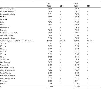
Summary statistics in 1982 and 2015 for modeled variables are summarized in Table 1. Between 1982 and 2015, interstate migration declined by nearly 50% (from 0.030 to 0.016), intrastate migration declined by 38% (from 0.034 to 0.021), and intracounty mobility declined by 30% (from 0.10 to 0.07). Figure 1 puts these trends in broader historical perspective and confirms that declines are not confined to interstate or local mobility. Furthermore, Figure 1 shows that these trends are not simply driven by the Great Recession. While recent drops in long-distance migration were offset by modest increases in local mobility during the recent recession and foreclosure crises (Stoll
2013), Figure 1 shows that this increase was temporary. As of 2015 local mobility rates were at an historic low of 7%.
Table 1: CPS summary statistics for modeled variables, 1982 and 2015
1982 2015
Mean SD Mean SD
Interstate migration 0.030 – 0.016 –
Intrastate migration 0.034 – 0.021 –
Intracounty mobility 0.101 – 0.070 –
NL White 0.816 – 0.649 –
NL Black 0.107 – 0.117 –
Latino 0.054 – 0.155 –
Other 0.024 – 0.079 –
Homeowner 0.721 – 0.670 –
Married 0.617 – 0.529 –
Dual earner household 0.292 – 0.284 –
Children present 0.428 – 0.368 –
4+ years of college 0.160 – 0.298 –
Total family income (1,000s of 1999 dollars) 45.799 34.120 56.032 63.207
18 to 24 0.177 – 0.124 –
25 to 34 0.235 – 0.178 –
35 to 44 0.166 – 0.165 –
45 to 54 0.136 – 0.177 –
55 to 64 0.133 – 0.167 –
65 to 74 0.095 – 0.111 –
75 and over 0.058 – 0.079 –
New England 0.057 – 0.047 –
Mid Atlantic 0.167 – 0.133 –
East North Central 0.182 – 0.148 –
West North Central 0.074 – 0.065 –
South Atlantic 0.163 – 0.198 –
East South Central 0.060 – 0.058 –
West South Central 0.102 – 0.115 –
Mountain 0.050 – 0.071 –
Pacific 0.145 – 0.163 –
N 113,295 144,279
Notes: Weighted CPS summary statistics for modeled variables.
With the exception of Total Family Income, summarized variables are bivariate dummies coded “1” to indicate the presence of a given characteristic and “0” to indicate its absence. The mean for these dummy variables, therefore, represents the proportion of the sample possessing the specified trait, and standard deviations are not reported.
roughly 27% (from 0.41 to 0.30), while the share of the population 45 and older increased 26% (from 0.42 to 0.53). These shifts contribute, to some degree, to overall declines in mobility and migration.
Figure 1: Annual mobility and migration trends, 1948–2015
Source: Current Population Survey annual mobility data.
Note: Quadratic curves are fit to the data to emphasize overall trends. Apparent jumps in mobility in 1985 reflect changes in CPS
sampling frames.
At the same time, other compositional shifts in favor of more mobile groups are clear in Table 1. The share of the sample married declined from 0.62 to 0.53, suggesting that a larger portion of the population is less tethered to place, and therefore more likely to move.7 Likewise, both the share of the population with four or more years of college
and the average total family income increased between 1982 and 2015. It is important to note the dramatic increase in the spread around the mean family income between 1982 and 2015. The widening distribution of incomes is consistent with the notion that earnings have stagnated at the middle and bottom of the distribution while inflating rapidly at the top. While the increasing share of dual-earner couples and homeowners is often cited as a cause of mobility and migration decline (Cooke 2013; Fischer 2002), this sample actually saw stagnating dual-earner and declining homeowner shares between 1982 and 2015. It is likely that these counterintuitive summary statistics are
influenced by the Great Recession and foreclosure crisis, which had enormous impacts on homeownership and employment in the United States. I return to the impact of the Great Recession later in the analysis.
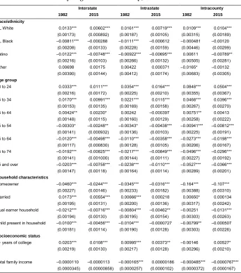
4.1 Stage one results: Predicting individual mobility in 1982 and 2015
Table 2: First stage Oaxaca–Blinder results for interstate, intrastate, and intracounty migration and mobility, 1982 and 2015
Interstate Intrastate Intracounty
1982 2015 1982 2015 1982 2015
Race/ethnicity
NL White 0.0133*** 0.00602*** 0.0161*** 0.00719*** 0.0109*** 0.0104***
(0.00173) (0.000892) (0.00187) (0.00105) (0.00315) (0.00189)
NL Black –0.00811*** –0.000288 –0.0111*** –0.000612 –0.000481 –0.00120
(0.00208) (0.00133) (0.00228) (0.00159) (0.00446) (0.00299)
Latino –0.0122*** –0.00748*** –0.00922*** –0.00695*** 0.00611 –0.00789**
(0.00216) (0.00103) (0.00266) (0.00132) (0.00505) (0.00281)
Other 0.00698 0.00175 0.00422 0.000371 –0.0165* –0.00132
(0.00390) (0.00144) (0.00412) (0.00174) (0.00683) (0.00305)
Age group
18 to 24 0.0333*** 0.0111*** 0.0354*** 0.0164*** 0.0848*** 0.0504***
(0.00216) (0.00172) (0.00225) (0.00210) (0.00355) (0.00367)
25 to 34 0.0170*** 0.00991*** 0.0221*** 0.0115*** 0.0468*** 0.0396***
(0.00153) (0.00135) (0.00169) (0.00158) (0.00267) (0.00270)
35 to 44 0.00424** 0.00230* 0.00242 –0.000397 0.00751** 0.00413
(0.00148) (0.00115) (0.00160) (0.00129) (0.00258) (0.00222)
45 to 54 –0.00303* –0.00248** –0.00343* –0.00438*** –0.00941*** –0.00812***
(0.00141) (0.000932) (0.00136) (0.00103) (0.00225) (0.00191)
55 to 64 –0.0120*** –0.00498*** –0.0110*** –0.00358*** –0.0273*** –0.0198***
(0.00117) (0.000830) (0.00128) (0.00105) (0.00206) (0.00167)
65 to 74 –0.0192*** –0.00825*** –0.0217*** –0.00849*** –0.0496*** –0.0296***
(0.00141) (0.001000) (0.00144) (0.00111) (0.00227) (0.00192)
75 and over –0.0203*** –0.00758*** –0.0238*** –0.0110*** –0.0527*** –0.0366***
(0.00147) (0.00118) (0.00164) (0.00114) (0.00289) (0.00201)
Household characteristics
Homeowner –0.0460*** –0.0244*** –0.0345*** –0.0316*** –0.164*** –0.107***
(0.00227) (0.00146) (0.00233) (0.00182) (0.00388) (0.00310)
Married 0.0173*** 0.00554*** 0.00666*** 0.000218 0.00650* 0.000134
(0.00195) (0.00131) (0.00200) (0.00136) (0.00317) (0.00242)
Dual earner household –0.0212*** –0.00716*** –0.00804*** –0.00462** –0.00251 –0.0131***
(0.00194) (0.00130) (0.00195) (0.00154) (0.00303) (0.00263)
Child present in household –0.0100*** –0.00456*** –0.0104*** –0.0000727 –0.00799** –0.000507
(0.00181) (0.00114) (0.00190) (0.00128) (0.00303) (0.00226)
Socioeconomic status
4+ years of college 0.0203*** 0.0108*** 0.00995*** 0.00373** –0.00146 0.00527*
(0.00219) (0.00130) (0.00217) (0.00128) (0.00296) (0.00210)
Total family income –0.0000110 –0.0000113 –0.000165*** 0.00000186 –0.000485*** –0.0000767***
Table 2: (Continued)
Interstate Intrastate Intracounty
1982 2015 1982 2015 1982 2015
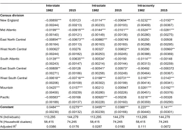
Census division
New England –0.00850*** 0.00123 –0.0114*** –0.00694*** –0.0232*** –0.0150***
(0.00244) (0.00213) (0.00233) (0.00193) (0.00409) (0.00367)
Mid Atlantic –0.0199*** –0.00915*** –0.0144*** –0.0101*** –0.0324*** –0.0281***
(0.00140) (0.00121) (0.00149) (0.00136) (0.00280) (0.00275)
East North Central –0.00854*** –0.00673*** –0.00860*** –0.000749 0.00250 0.00508
(0.00164) (0.00113) (0.00163) (0.00160) (0.00298) (0.00295)
West North Central 0.000627 0.00276 0.00327 0.00802** 0.00290 0.00960**
(0.00244) (0.00182) (0.00253) (0.00245) (0.00386) (0.00369)
South Atlantic 0.0139*** 0.00635*** 0.00534* –0.00190 –0.0114*** –0.00148
(0.00243) (0.00147) (0.00214) (0.00144) (0.00313) (0.00259)
East South Central –0.00809** –0.00128 –0.00541* 0.00573* –0.00492 –0.000372
(0.00271) (0.00186) (0.00258) (0.00248) (0.00464) (0.00367)
West South Central –0.00618** –0.00716*** 0.0199*** 0.00731*** 0.0187*** 0.0143***
(0.00206) (0.00109) (0.00302) (0.00199) (0.00414) (0.00341)
Mountain 0.0425*** 0.0157*** 0.00213 0.000947 0.0261*** 0.0192***
(0.00400) (0.00239) (0.00280) (0.00226) (0.00451) (0.00376)
Pacific –0.00583** –0.00168 0.00920*** –0.00236 0.0216*** –0.00326
(0.00189) (0.00137) (0.00228) (0.00160) (0.00359) (0.00290)
Constant 0.0484*** 0.0279*** 0.0495*** 0.0388*** 0.220*** 0.141***
(0.00230) (0.00132) (0.00239) (0.00166) (0.00440) (0.00301)
N (Individuals) 113,295 144,279 113,295 144,279 113,295 144,279
N (Household clusters) 58,415 74,245 58,415 74,245 58,415 74,245
Adjusted R2 0.0386 0.0176 0.0287 0.0180 0.111 0.0672
Notes: *p<0.05; **p<0.01; ***p<0.001. t-statistics in parentheses
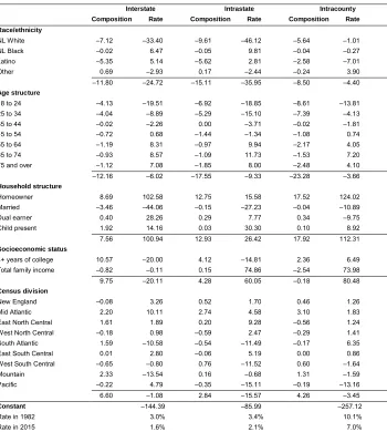
4.2 Stage two results: Compositional components of migration and mobility decline between 1982 and 2015
have been higher than observed, while positive values indicate that counterfactual rates would have been lower.
Table 3: Second stage Oaxaca–Blinder decomposition results, 1982 to 2015
Interstate Intrastate Intracounty
Composition Rate Composition Rate Composition Rate
Race/ethnicity
NL White –7.12 –33.40 –9.61 –46.12 –5.64 –1.01
NL Black –0.02 6.47 –0.05 9.81 –0.04 –0.27
Latino –5.35 5.14 –5.62 2.81 –2.58 –7.01
Other 0.69 –2.93 0.17 –2.44 –0.24 3.90
–11.80 –24.72 –15.11 –35.95 –8.50 –4.40
Age structure
18 to 24 –4.13 –19.51 –6.92 –18.85 –8.61 –13.81
25 to 34 –4.04 –8.89 –5.29 –15.10 –7.39 –4.13
35 to 44 –0.02 –2.26 0.00 –3.71 –0.02 –1.81
45 to 54 –0.72 0.68 –1.44 –1.34 –1.08 0.74
55 to 64 –1.19 8.31 –0.97 9.94 –2.17 4.05
65 to 74 –0.93 8.57 –1.09 11.73 –1.53 7.20
75 and over –1.12 7.08 –1.85 8.00 –2.48 4.10
–12.16 –6.02 –17.55 –9.33 –23.28 –3.66
Household structure
Homeowner 8.69 102.58 12.75 15.58 17.52 124.02
Married –3.46 –44.06 –0.15 –27.23 –0.04 –10.89
Dual earner 0.40 28.26 0.29 7.77 0.34 –9.75
Child present 1.92 14.16 0.03 30.30 0.10 8.92
7.56 100.94 12.93 26.42 17.92 112.31
Socioeconomic status
4+ years of college 10.57 –20.00 4.12 –14.81 2.36 6.49
Total family income –0.82 –0.11 0.15 74.86 –2.54 73.98
9.75 –20.11 4.28 60.05 –0.18 80.48
Census division
New England –0.08 3.26 0.52 1.70 0.46 1.26
Mid Atlantic 2.20 10.11 2.74 4.58 3.10 1.83
East North Central 1.61 1.89 0.20 9.28 –0.56 1.24
West North Central –0.18 0.98 –0.59 2.47 –0.29 1.41
South Atlantic 1.59 –10.58 –0.54 –11.49 –0.17 6.35
East South Central 0.01 2.80 –0.06 5.19 0.00 0.86
West South Central –0.65 –0.80 0.76 –11.52 0.60 –1.64
Mountain 2.33 –13.54 0.16 –0.68 1.31 –1.59
Pacific –0.22 4.79 –0.35 –15.11 –0.19 –13.16
6.60 –1.08 2.84 –15.57 4.26 –3.45
Constant –144.39 –85.99 –257.12
Rate in 1982 3.0% 3.4% 10.1%
Rate in 2015 1.6% 2.1% 7.0%
Changes in the age structure of the US population account for 12% of interstate migration decline, 18% of intrastate migration decline, and 23% of intracounty mobility decline between 1982 and 2015. Most of this age effect is attributable to significant declines in the population share under age 34 (Table 1). These results are consistent with several other studies that find substantial population aging effects. In their study of interstate migration decline since the mid-1980s, Karahan and Rhee (2014) find that about half of all interstate migration decline is attributable to population aging. Roughly 75% of this effect is direct, in that migration typically declines with age (e.g., Table 2), while the remaining 25% is attributable to age-group spillover effects, by which growth in the middle-aged working population (those 40 to 60) in a state reduces the migration rates of all other workers as well. In this light, the estimate shown in Table 3 that 12% of all interstate migration decline is due to population aging may be conservative. At the intrastate and intracounty levels the contribution of aging to declines reported here is consistent with other studies, which show considerable age effects on shorter-distance migration and local mobility (Cooke 2011; Molloy, Smith, and Wozniak 2011, 2014).
In the counterfactual absence of increasing racial and ethnic diversity, annual rates of interstate, intrastate, and intracounty movement would have been 12%, 15%, and 9% higher than actually observed. Because non-Latino White populations tend to move at higher rates (Table 2), most of the diversity effect is attributable to this group: shrinking non-Latino White shares are associated with 7% of interstate, 10% of intrastate, and 6% of intracounty declines. Substantial growth in the Latino population, a typically less mobile group, is associated with over 5% of interstate and intrastate declines. Taken together with population aging, these results suggest that roughly 32% of all intracounty mobility, 33% of all intrastate migration, and 24% of interstate migration declines between 1982 and 2015 are attributable to what some scholars are calling the Third Demographic Transition (Coleman 2006; Lichter 2013).
decline, Table 3 shows negligible dual-earner effects and positive homeowner effects. As noted above, the homeowner shares actually decreased between 1982 and 2015 (Table 1), likely due to the impact of the Great Recession and foreclosure crisis of the mid and late 2000s. Because homeowners are less likely to move than their renting and single-earner counterparts (Table 2), declining homeowner shares between 1982 and 2015 are associated with 9%, 13%, and 18% increases in interstate, intrastate, and intracounty movement, respectively.
4.3 The impact of the Great Recession and foreclosure crisis
There are reasons to suspect that the economic downturn in the mid-2000s biases the decomposition results discussed thus far. In his decomposition of intercounty migration decline between 1999 and 2009, Cooke (2011) found that more than 60% of all declines were attributable to the foreclosure crisis and resulting recession. It is important to note, however, that while the recession appears to have contributed to declines in longer-distance interstate and intercounty migration, it temporarily increased rates of local intracounty mobility (Stoll 2013).
The central goal of this paper is to understand how broader shifts in the US population have contributed to migration and mobility decline over the long-term. The overwhelming effects of the Great Recession on migration and mobility cloud this broader understanding, so I replicate the above analysis for the pre-recession 1982 to 2006 period. Second-stage results of this supplemental analysis are presented in Table 4.
Table 4: Second stage Oaxaca–Blinder decomposition results, 1982 to 2006
Interstate Intrastate Intracounty
Composition Rate Composition Rate Composition Rate
Race/ethnicity
NL White ‒4.68 ‒58.31 ‒20.52 ‒75.35 ‒2.55 ‒23.38
NL Black 0.16 11.48 ‒0.47 12.92 0.01 0.49
Latino ‒7.23 2.13 ‒9.92 3.68 1.07 ‒2.14
Other 1.16 ‒2.14 1.49 ‒2.16 ‒1.44 2.84
‒10.59 ‒46.85 ‒29.42 ‒60.91 ‒2.91 ‒22.18
Age structure
18 to 24 ‒9.18 ‒15.64 ‒19.97 ‒27.24 ‒16.15 ‒13.02
25 to 34 ‒6.03 ‒8.72 ‒15.41 ‒19.31 ‒14.10 3.24
35 to 44 0.87 ‒1.99 2.53 8.35 1.32 1.26
45 to 54 ‒1.93 ‒0.91 ‒4.02 ‒1.65 ‒3.50 ‒2.32
55 to 64 ‒0.51 6.68 ‒1.29 4.27 ‒1.01 1.43
65 to 74 1.16 5.84 2.58 11.63 2.06 4.96
75 and over ‒2.28 5.38 ‒5.68 9.21 ‒4.73 1.61
‒17.89 ‒9.37 ‒41.26 ‒14.74 ‒36.11 ‒2.84
Household structure
Homeowner ‒0.06 97.38 ‒0.14 ‒42.75 ‒0.13 153.11
Married ‒4.05 ‒50.52 ‒1.54 ‒49.87 0.61 ‒24.08
Dual earner ‒2.93 26.85 ‒3.40 3.23 ‒1.50 ‒14.11
Child present 0.99 25.43 3.00 38.08 ‒0.30 19.04
‒6.06 99.15 ‒2.09 ‒51.31 ‒1.32 133.97
Socioeconomic status
4+ years of college 8.36 ‒25.45 8.23 ‒22.08 1.29 5.33
Total family income ‒0.07 5.47 ‒3.77 145.10 ‒5.56 111.26
8.29 ‒19.98 4.46 123.02 ‒4.27 116.58
Census division
New England 0.15 2.88 1.40 0.79 0.67 1.41
Mid Atlantic 3.14 10.19 5.17 9.49 3.72 4.51
East North Central 1.02 6.29 1.03 17.18 0.00 ‒1.98
West North Central ‒0.27 2.46 ‒0.69 3.48 ‒0.02 ‒0.80
South Atlantic 2.21 ‒10.70 4.22 8.90 ‒0.98 4.82
East South Central 0.02 2.82 0.04 1.66 ‒0.01 2.81
West South Central ‒0.18 3.16 1.91 ‒5.74 0.15 ‒7.66
Mountain 3.08 ‒15.32 ‒0.32 ‒3.74 3.42 3.86
Pacific ‒0.90 ‒1.14 ‒0.79 ‒34.09 0.21 ‒15.15
8.27 0.65 11.97 ‒2.06 7.16 ‒8.18
Constant ‒98.65 9.32 ‒249.04
Rate in 1982 3.0% 3.4% 10.1%
Rate in 2006 2.0% 2.8% 8.1%
Notes: Results of Oaxaca–Blinder Decomposition. Effects reported as a percentage contribution to observed aggregate declines between 1982 and 2006. Totals under horizontal lines for each section report the sum contribution of effects in that section.
2006 homeownership remained relatively stable at 72% and dual-earner household shares increased from 29% to 32%. As such, the 2006 endpoint allows a more direct test of the long-term impact of homeownership and dual-earner couples in the United States on aggregate migration trends. Slight increases in homeownership rates between 1982 and 2006 do, in fact, contribute to migration and mobility declines over this period, but these effects account for less than 1% of all declines. Similarly, increasing dual-earner shares in the pre-Great Recession period promote immobility, but account for only 3% of interstate and intrastate migration declines, and only 1.5% of local mobility declines. Relative to other compositional shifts, then, rising homeownership rates and dual-earner shares have a negligible influence on the aggregate mobility and migration patterns of Americans.
4.4 Rate components of mobility and migration decline: Age, race, and geography
Discussion thus far has focused on the compositional effects presented in Tables 3 and 4. To a large extent, this narrow focus is justified in the larger literature on American mobility decline, which to date has been reluctant to acknowledge substantial demographic, socioeconomic, and regional differences in the timing, rate, and magnitude of declining mobility. Instead, studies to date stress the universality of declining rates of mobility and migration across nearly all racial and ethnic groups and therefore overlook the possibility that region- or group-specific causes of immobility may play a role.
The rate effects reported in Tables 3 and 4 gauge the contribution of changing coefficients associated with individual characteristics from stage one of the decomposition. A negative rate effect reflects a net decline between 1982 and 2015 in movement for individuals with a given characteristic, while a positive rate effect reflects increased movement. Put another way, a negative rate effect suggests that in the counterfactual absence of a change in the rate at which individuals with a given characteristic move, aggregate rates would have been higher (and vice versa for positive rate effects).
(2016) recent analysis of mobility trends among householders in the Panel Study of Income Dynamics, which finds much more dramatic declines among renters than among homeowners. These rate effects are so large that at the interstate and intracounty levels they are equal to the observed declines in migration and mobility since 1982. Put another way, in the counterfactual scenario in which rates of decline were the same for homeowners as for renters, overall declines in migration and mobility may have been only half as large as those actually observed. There are similar, though smaller, positive rate effects over longer distances among Blacks, Latinos, and dual-earners. While stagnant dual-earner household shares between 1982 and 2015 did not have a large compositional effect on declines, rate effects are compelling. Rates of interstate migration among dual-earner couples declined much less rapidly between 1982 and 2015 than among their single-earner counterparts.
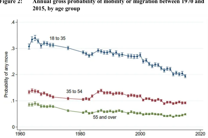
Figure 2: Annual gross probability of mobility or migration between 1970 and 2015, by age group
Note: Predicted probabilities from bivariate logistic regression of CPS annual mobility data are shown with 95% confidence intervals.
Data are only available periodically in the 1970s.
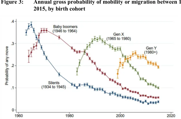
seven-category age structure modeled in the analyses above into three categories: 18 to 34, 35 to 54, and 55 years of age and older. As these trend lines demonstrate, both the overall magnitude of declines and the rate of declines are much greater for those 18 to 35 years of age than for those 35 and older. Moreover, while those over age 35 show some signs of rising mobility rates since 2010, rates for those under 35 continue to decline. Figure 3 offers a cohort or generational perspective on age-specific rate effects, plotting mobility rates across the life course for four birth cohorts: the Silent Generation (born 1934–1945); Baby Boomers (born 1946–1964); Gen X (born 1965–1980); and the Gen Y or Millennial Generation (born after 1980). The cohort perspective demonstrates clearly the decline in mobility among those under 35: each successive generation reaches peak rates of mobility later in life – at 20 years of age in the Silent Generation, but at 23 years for Baby Boomers, 24 years for Generation X, and 25 years for Millennials – and those peak rates decline with each successive generation. These findings contradict Plane and Rogerson’s (1991) prediction that mobility among the young would increase through the turn of the 21st century. As such, declining mobility
among younger age groups appears to be driven by broader generational shifts in mobility and migration patterns, which may be related to the increasing barriers to labor market entry and the increasing debts incurred earning a college education (Cooke 2013). This conclusion is supported by decomposition results in Table 3 that show sharply declining migration rates among those with a college education. Though growth in the typically more mobile college-educated population offsets declines, rates of interstate and intrastate migration in this population account for 20% and 15% of declines, respectively.
Figure 3: Annual gross probability of mobility or migration between 1962 and 2015, by birth cohort
Note: Predicted probabilities from bivariate logistic regression of CPS annual mobility data are shown with 95% confidence intervals.
Only those 18 years of age and older are included. Data are only available periodically in the 1970s.
Figure 4: Annual gross probability of mobility or migration between 1970 and 2015, by race/ethnicity
Note: Predicted probabilities from bivariate logistic regression of CPS annual mobility data are shown with 95% confidence intervals.
The rapid decline in Latino White mobility and migration relative to non-Latino African Americans is depicted graphically in Figure 4, which tracks the gross probability of any move between 1970 and 2015.8 Mobility rates for both White and
Black Americans peaked in the late 1980s but have declined precipitously since then. The rate of decline among non-Latino Whites is more dramatic than that of African Americans, however, resulting in a growing racial gap in aggregate mobility (Carll et al. 2016). These racial and ethnic differences in longer-distance migration decline are consistent with findings outside of the narrow migration decline literature (e.g., Sharkey 2013, 2015) and hold important implications for studies of racial and ethnic inequality in the United States (Carll et al. 2016; Foster 2017).
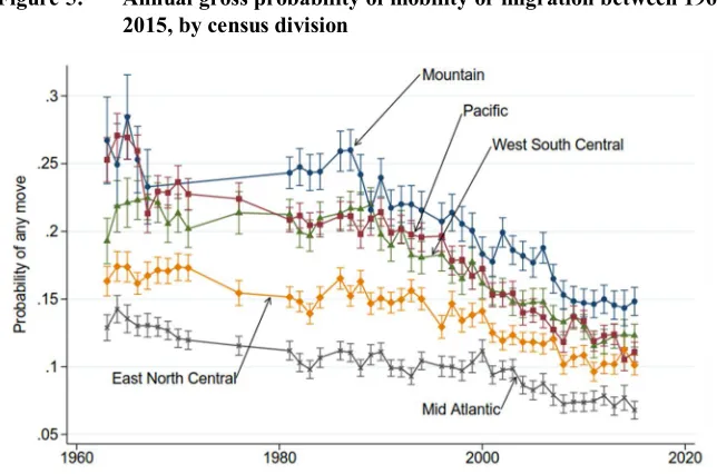
Figure 5: Annual gross probability of mobility or migration between 1962 and 2015, by census division
Note: Predicted probabilities from bivariate logistic regression of CPS annual mobility data are shown with 95% confidence intervals.
Data are only available periodically in the 1970s. Not shown are trend lines for New England, West North Central, South Atlantic, and East South Central regions.
Rate effect results also reveal sizeable regional variations in rates of decline that appear to reflect population shifts from the Rustbelt to the Sunbelt (Frey 2002; Iceland, Sharp, and Timberlake 2013). Trends in the probability of any move originating in each
census division are shown in Figure 5. While migration has declined in all regions, declines are steeper in the South and West: these particularly pronounced declines are reflected in the relatively large negative rate effects reported in Tables 3 and 4 for Pacific, Mountain, and West South Central regions. Declines in the Mid-Atlantic and East North Central regions are notably less dramatic than the grand mean, as reflected by the positive rate effects in Tables 3 and 4. Taken together, these trends and results are consistent with sustained out-migration from former manufacturing centers in the Rustbelt Northeast and Midwest and population growth in the Sunbelt South and West. Further supporting this view is the relatively high level of local mobility in the South Atlantic region, which may reflect population churning associated with high levels of in-migration (Frey 1978). More research into the geographic structure of migration decline is sorely needed, however.
5. Conclusion
This research contributes to the emerging literature on American mobility and migration decline since the mid-20th century by gauging the contribution of population
composition shifts to overall declines and by addressing two shortcomings of prior research. First, prior analyses of the role of compositional change were limited in temporal scope. I remedy this by decomposing aggregate migration and mobility rates between 1982 and 2015 using consistent measures of mobility in the IPUMS-CPS. Second, prior analyses have not systematically addressed how compositional shifts might influence migration and local mobility in different ways. I remedy this by decomposing changes in three different types of movement: long-distance migration between states, medium-distance migration between counties in the same state, and short-distance mobility within the same county.
Population aging and increasing ethnoracial diversity contribute to rising American immobility, accounting for roughly one-quarter to one-third of all declines in migration and mobility. Partially offsetting these declines is the growing share of the population with a college education. Generally speaking, increasing ethnoracial diversity and rising education levels exert a larger influence on long-distance migration, while population aging has a larger immobilizing impact on local mobility. Though they are often cited as important contributors to rising immobility, the results presented here suggest that changes in homeownership and dual-earner household shares exert a negligible impact on the changing mobility and migration patterns of Americans, even prior to the Great Recession and foreclosure crisis of 2007.
revealed in this decomposition. While migration and mobility have fallen for nearly all Americans (Fischer 2002), they have fallen much more rapidly in portions of the South and West, as well as among non-Latino Whites and those under age 35. A descriptive birth cohort analysis of mobility across the life-course shows that the peak migration rate for each successive cohort occurs later and peaks lower than the last. These findings suggest that broad social and economic shifts since the mid-20th century may
disproportionately affect younger Americans and, broadly speaking, may be more important for our nascent understanding of rising immobility.
This work is not without its limitations. First, as is clear from prior studies of mobility and migration decline, results are sensitive to the periods studied. In this paper I addressed a major source of sensitivity, the Great Recession of the mid-2000s, by examining declines over two periods of time, from 1982 to 2006 and from 1982 to 2015. As such, analysis was able to isolate long-term composition effects from noise introduced by recession-related economic declines. Second, the retrospective nature of the CPS mobility item means that most of the individual-level covariates used in the preceding analyses are measured after mobility or migration occurs. It is possible to overcome this problem by linking observations for the same individual across monthly iterations of the CPS, but this process is quite difficult, especially in earlier CPS samples (Rivera-Drew, Flood, and Warren 2014). Imprecision introduced by this necessary limitation, however, likely biases the estimates presented here downward. That is, if estimates are affected at all by measuring characteristics at the end of a mobility interval rather than at the beginning, they likely underestimate the true effects.
most worrisome. The results presented here hint at the possibility that Americans may be increasingly constrained in their mobility and migration choices (Sharkey 2013, 2015), and increasingly unable to overcome the costs or reap the benefits associated with moving (Seelye 2016). In short, and contrary to the predominant conclusion in the emerging literature, rising immobility may indicate that Americans are increasingly stuck, rather than rooted.
6. Acknowledgments
References
Blinder, A.S. (1973). Wage discrimination: Reduced form and structural estimates.
Journal of Human Resources 8(4): 436–455.doi:10.2307/144855.
Carll, E., Foster, T.B., and Crowder, K. (2016). Converging rates, divergent trajectories? Race- and gender-based stratification in Renters’ residential mobility from 1970 to 2011. Paper presented at the Annual Meeting of the Population Association of America, Washington D.C., US, March 28–April 2, 2016.
Chetty, R., Hendren, N., Kline, P., and Saez, E. (2014). Where is the land of Opportunity? The geography of intergenerational mobility in the United States.
The Quarterly Journal of Economics 129(4): 1553–1623.doi:10.3386/w19843. Coleman, D. (2006). Immigration and ethnic change in low-fertility countries: A third
demographic transition. Population and Development Review 32(3): 401–446. doi:10.1111/j.1728-4457.2006.00131.x.
Cooke, T.J. (2011). It is not just the economy: Declining migration and the rise of secular rootedness: Secular rootedness.Population, Space and Place 17(3): 193– 203.doi:10.1002/psp.670.
Cooke, T.J. (2013). Internal migration in decline.The Professional Geographer 65(4): 664–675.doi:10.1080/00330124.2012.724343.
Cooke, T.J., Mulder, C.H., and Thomas, M. (2016). Union dissolution and migration.
Demographic Research 34(26): 741–760.doi:10.4054/DemRes.2016.34.26. Crowder, K. and South, S.J. (2005). Race, class, and changing patterns of migration
between poor and nonpoor neighborhoods. American Journal of Sociology
110(6): 1715–1763.doi:10.1086/428686.
Fischer, C. (2002). Ever-more rooted Americans. City and Community 1(2): 177–198. doi:10.1111/1540-6040.00016.
Flood, S., King, M., Ruggles, S., and Warren, J.R. (2015). Integrated Public Use Microdata Series, Current Population Survey: Version 4.0 [electronic resource]. Minneapolis: University of Minnesota.https://cps.ipums.org/cps/.
Foster, T.B. (2017). The persistent black-white gap in and weakening link between expecting to move and actually moving. Sociology of Race and Ethnicity. doi:10.1177/2332649217728374.
Frey, W.H. (1978). Population movement and city-suburb redistribution: An analytic framework.Demography 15(4): 571–588.doi:10.2307/2061208.
Frey, W.H. (2002). Three Americas: The rising significance of regions.Journal of the American Planning Association 68(4): 349–355. doi:10.1080/0194436020897 6279.
Frey, W.H. (2015). Diversity explosion: How new racial demographics are remaking America. Washington, D.C.: Brookings Institution Press.
Greenwood, M.J. (1975). Research on internal migration in the United States: A survey.
Journal of Economic Literature 13(2): 397–433.
Greenwood, M.J. (1985). Human migration: Theory, models, and empirical studies.
Journal of Regional Science 25(4): 521–544.doi:10.1111/j.1467-9787.1985.tb0 0321.x.
Greenwood, M.J. (1997). Internal migration in developed countries. In: Rosenzweig, M. and Stark, O. (eds.).Handbook of population and family economics. Amsterdam: Elsevier: 647–720.doi:10.1016/S1574-003X(97)80004-9.
Harrison, B. and Bluestone, B. (1988).The great U-turn: Corporate restructuring and the polarizing of America. New York: Basic Books.
Harvey, D. (2010).The enigma of capital and the crises of capitalism. London: Profile Books.
Herting, J.R., Grusky, D.B., and Van Rompaey, S.E. (1997). The social geography of interstate mobility and persistence. American Sociological Review 62(2): 267– 287.doi:10.2307/2657304.
Hobbs, F. and Stoops, N. (2002). Demographic trends in the 20th century. Washington, D.C.: US Census Bureau (Census 2000 Special Reports, Series CENSR-4). Iceland, J., Sharp, G., and Timberlake, J.M. (2013). Sun Belt rising: Regional
population change and the decline in black residential segregation, 1970–2009.
Demography 50(1): 97–123.doi:10.1007/s13524-012-0136-6.
Kaplan, G. and Schulhofer-Wohl, S. (2012). Understanding the long-run decline in interstate migration. Cambridge: National Bureau of Economic Research (NBER Working Paper 18507).doi:10.3386/w18507.
Karahan, F. and Rhee, S. (2014). Population aging, migration spillovers, and the decline in interstate migration. New York: Federal Reserve Bank of New York (FRB-NY Staff Report 699).
Lee, E. (1966). A theory of migration.Demography 3(1): 47–57.doi:10.2307/2060063. Lesthaeghe, R.J. and Neidert, L. (2006). The second demographic transition in the
United States: Exception or textbook example? Population and Development Review 32(4): 669–698.doi:10.1111/j.1728-4457.2006.00146.x.
Lichter, D.T. (2013). Integration or fragmentation? Racial diversity and the American future.Demography 50(2): 359–391.doi:10.1007/s13524-013-0197-1.
Long, L. (1988). Migration and residential mobility in the United States. New York: Russell Sage Foundation.
Massey, D.S. (1996). The age of extremes: Concentrated affluence and poverty in the twenty-first century.Demography 33(4): 395–412.doi:10.2307/2061773. Molloy, R., Smith, C.L., and Wozniak, A.K. (2011). Internal migration in the United
States.Journal of Economic Perspectives 25(3): 173–196.doi:10.3386/w17307. Molloy, R., Smith, C.L., and Wozniak, A.K. (2014). Declining migration within the
US: The role of the labor market. Bonn: Institute of Labor Economics (IZA Discussion Paper 8149).doi:10.3386/w20065.
Molloy, R., Smith, C.L., and Wozniak, A.K. (2017). Job changing and the decline in long-distance migration in the United States. Demography 54(2): 631–653. doi:10.1007/s13524-017-0551-9.
Mueser, P. (1989). The spatial structure of migration: An analysis of flows between states in the USA over three decades. Regional Studies 23(3): 185–200. doi:10.1080/00343408912331345412.
Oaxaca, R.L. (1973). Male-female wage differentials in urban labor markets.
International Economic Review 14(3): 693–709.doi:10.2307/2525981.
Plane, D.A. and Rogerson, P.A. (1991). Tracking the baby boom, the baby bust, and the
echo generations: How age composition regulates US migration. The
Reich, R.A. (2010). Aftershock: The next economy and America’s future. New York: Knopf.
Rivera-Drew, J.A., Flood, S., and Warren, J.R. (2014). Making full use of the longitudinal design of the Current Population Survey: Methods for linking records across 16 months. Journal of Economic and Social Measurement 39(3): 121–144.
Ritchey, P.N. (1976). Explanations of migration.Annual Review of Sociology 2: 363– 404.doi:10.1146/annurev.so.02.080176.002051.
Rogers, A. and Sweeney, S. (1998). Measuring the spatial focus of migration patterns.
The Professional Geographer 50(2): 232–242.doi:10.1111/0033-0124.00117. Rogers, A., Willekens, F., Little, J., and Raymer, J. (2002). Describing migration spatial
structure. Papers in Regional Science 81(1): 29–48. doi:10.1111/j.1435-5597. 2002.tb01220.x.
Rosenfeld, J. (2014).What unions no longer do. Cambridge: Harvard University Press. doi:10.4159/harvard.9780674726215.
Seelye, S.M. (2016). Staying put in Detroit’s high-poverty neighborhoods. Paper presented at the Annual Meeting of the Population Association of America, Washington, D.C., US, March 28–April 2, 2016.
Sharkey, P. (2013). Stuck in place: Urban neighborhoods and the end of progress toward racial equality. Chicago: University of Chicago Press. doi:10.7208/ chicago/9780226924267.001.0001.
Sharkey, P. (2015). Geographic migration of black and white families over four generations.Demography 52(1): 209–231.doi:10.1007/s13524-014-0368-8. South, S.J. and Crowder, K. (1997). Escaping distressed neighborhoods: Individual,
community, and metropolitan influences.American Journal of Sociology 102(4): 1040–1084.doi:10.1086/231039.
Spring, A., Tolnay, S., and Crowder, K. (2016). Moving for opportunities? Changing patterns of migration in North America. In: White, M.J. (ed.). International handbook of migration and population. Dordrecht: Springer: 421–448. doi:10.1007/978-94-017-7282-2_19.
Vaupel, J.W. and Canudas-Romo, V. (2002). Decomposing demographic change into direct vs. compositional components. Demographic Research 7(1): 1–14. doi:10.4054/DemRes.2002.7.1.
Western, B. and Rosenfeld, J. (2011). Unions, norms, and the rise in American wage inequality. American Sociological Review 76(4): 513–537. doi:10.1177/ 0003122411414817.