* Corresponding author. fax: +98-21-77240482 E-mail addresses: [email protected](A. Jamili) © 2011 Growing Science Ltd. All rights reserved. doi: 10.5267/j.ijiec.2010.03.005
Contents lists available at GrowingScience
International Journal of Industrial Engineering Computations
homepage: www.GrowingScience.com/ijiec
A new mathematical model for the job shop scheduling problem with uncertain processing times
M. A. Shafiaa , M. Pourseyed Aghaeeband A. Jamilia*
aDepartment of Industrial Engineering, Iran University of Science and Technology, Tehran Iran
bDepartment of Railroad Engineering ,Iran University of Science and Technology, Tehran, Iran
A R T I C L E I N F O A B S T R A C T
Article history: Received 1 Feb 2010 Received in revised form 10 June 2010
Accepted 20 June 2010 Available online 23 June 2010
Job shop scheduling (JSS) problem has been one of the most interesting research issues in the literature during the recent years. JSS problem has been studied in different forms of deterministic, fuzzy, and stochastic at different depths. The idea of robust optimization (ROP), on the other hand, has earned a particular value to become a popular subject of the breakthrough for problem solving affairs amongst the researchers. Based on the emerged opportunity for illustrating a new area of search, a robust JSS problem is proposed as a challenge to this boundary of knowledge. The proposed method is capable of handling the perturbation which exists amongst the processing times. In fact, in many real world job scheduling problems, a small change in the processing times, not only causes a non-optimal solution, but also the infeasibility of the final solution may also occur. The proposed robust method could guarantee that, a small deviation of the processing times does not affect the feasibility. The implementation of the proposed method is illustrated using some numerical examples and the outcomes of the investigation are discussed
©2011 Growing Science Ltd. All rights reserved.
Keywords:
Job Shop Scheduling Robust optimization Simulated annealing Heuristic
Mixed Integer Programming Uncertainty
Interruption
1. Introduction
(2000) presented a more popular robust approach which addressed a more conservative solution where a non-linear robust optimization model is presented. Bertsimas and Sim (2004) introduced a new robust approach in which the robust counterpart is of the same class as the nominal problem and therefore the proposed robust approach remains linear/mixed integer, if the nominal problem is linear/mixed integer.
Consider a linear constraint i
j
ij
ij x b
a × ≤
∑
and let Jirepresent the set of coefficients which aresubject to perturbation (aij, j∈Ji). The true value a~ equals ij
(
1+εξij)
aij whereε
>0 is a givenuncertainty level and ξij are random variables distributed symmetrically in the interval [-1, 1].
Thereforea~ , ij j∈Ji takes values in
[
aij−ˆaij,aij +ˆaij]
. Bertsimas and Sim (2004) proposed parameteri
i ≤ J
Γ ≤
0 , to adjust the desired conservatism level of the final solution. It means that at last only
⎣ ⎦
Γi are allowed to change, and one coefficient aitichanges by(
Γi−⎣ ⎦
Γi)
aˆiti.Note that, if Γi = Ji is considered, the method is reduced to Soyster’s approach. The idea of using
robust optimization has become popular (Farhang Moghadam & Seyed Hosseini, 2010; Gharakhani et al., 2010; Roghanian & Foroughi, 2010). For more details on the implementation of robust optimization, interested readers are referred to (Bertsimas & Sim, 2004). Shafia et al., (2010) adapted the latter approach to train routing and makeup problem.
2. Robust Job Shop Problem
As we explained, the perturbation is normally occurs in JSS problem, especially in the processing times of jobs in each machine. Suppose one is about to schedule the job shop problem introduced by Baker (1974). The tabular representations of the data for this prototype problem are shown in Table 1.a and Table 1.b.
Table 1.a
Processing Times
Table1.b
Routing
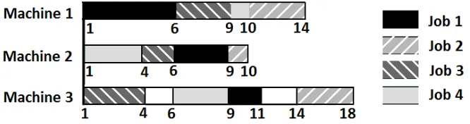
Consider minimization of total weighted tardiness (TWT) as the objective function, and let the starting time of schedule for each job, release time, to be equal to 1. The optimal solution for this example is shown as Fig. 1. Furthermore it is noticeable that this solution is also optimal in the case of makespan objective.
Operation 1 2 3
Job
1 4 3 2
2 1 4 4
3 3 2 3
4 3 3 1
Operation 1 2 3
Job
1 1 2 3
2 2 1 3
3 3 2 1
Fig. 1. Optimal Job Shop Schedule
As we can observe from Fig. 1, the optimum schedule value is 10. One can assume that the operation of job 1 in machine 1 is subjected to perturbation and the processing time is increased by one. In other words it changes from 4 to 5. This alteration makes the solution shown in Fig. 1, non-optimal. The perturbed schedule is depicted in Fig. 2.
Fig. 2. Perturbed Job Shop Schedule
As it can be found in Fig 2, this interruption worsens the TWT by 3 minutes (10→13). However, for
this case the optimum schedule on the basis of TWT is calculated as Fig. 3.
Fig. 3. Optimal Job Shop Schedule-perturbation case
The optimum schedule value in Fig. 3 for the TWT objective function is 10. It can be easily verified that just a little perturbation can highly change the optimum solution and this could be regarded as a good motivation to the robust optimization concept.
In the remaining part of this section, the robust JSS problem is introduced after proposing an appropriate mathematical model for the classical JSS problem. At the first step, the reader can consider the integer programming model specified by Baker. The employed notations are as follows:
Notations
A: Set of machines,
{
1,2,..,.m}
P: Set of jobs,
{
1,2,..,.n}
pjm
t : Required time to process task j of job p on machine m
i
e : The machine which performs the last operation on job i
M: A big number
pm
ipm
b : A binary variable which is 1, if job i precedes job p on machine m and 0, otherwise
Model 1:
∑
∈P i
iei
a
min
subject to:
ijk ih
ik a t
a − ≥ ,
(
i,j−1,h) (
<< i,j,k)
(1)(
ipk)
pqk ikpk a M b t
a − + 1− ≥ , i,p∈P, k∈A (2)
ijk ipk pk
ik a M b t
a − + × ≥ , i,p∈P, k∈A (3)
0
≥
ik
a , i∈P, k∈A
{ }
0,1∈
ipk
b , i,p∈P, k∈A
See (Baker, 1974) for more details.
Since, the processing times,tpjm, is subject to perturbation, the introduced robust method must be
applied on inequalities 1, 2 and 3. It can be observed that for all these equations, there is only one perturbed parameter in each constraint. As a result by applying the introduced robust approach to these inequalities, the achieved results are the same as solving the model in the worst-case, where a fix supplementary time is added to all processing times. On the other hand, it is clear that model 1 is only capable to cover the effects of possible perturbation amongst the consecutive jobs. Therefore, in this case, the effects of perturbation propagation amongst jobs are ignored. In order to overcome the mentioned weak characteristics, another formulation is proposed in which the sequencing of jobs on machines is appeared in the model. Following notations are used for the proposed model 2.
Notations
s: Sequence index defined for each job in every machine
Op: The last operation associated with job p.
jpms
x : A binary variable which is 1, if task j of job p is allocated on machine m in sequence
s, and 0, otherwise.
jpms
y : Denotes start-processing time of task j of job p on machine m
ms
L : Denotes the idle time of machine m in sequence s. i.e. the gap between (s)-th and
(s-1)-th operations performed on machine m.
Model 2:
∑ ∑∑
(
)
∈ ∈ =
=
P
p m A
P
s Oppms
y Z
1
min (4)
subject to:
∑∑
= ∈
=
P
s m A jpms
x 1
,
1 ∀j,p (5)
∑∑
∈ =
≤
P p
O
j jpms
p x 1
1 , ∀m,s (6)
jpms
jpms M x
y ≤ × , ∀j,p,m,s (7)
(
)
∑ ∑
∑ ∑
= ∈ = ∈ +
≤ × +
P
s m A
P
s m A
pms j jpm
jpms
jpms x t y
y
1 1
) 1
( , ∀j,p (8)
(
)
∑∑
∑∑
∈ = +
∈ =
≤ × +
P p
O
j jpms
P p
O
j jpms jpms jpm
p p
y t
x y
1 1
1
The objective function shown in equation 4 minimizes the sum of finishing time of the last operation of each job. Eq. 5 indicates that task j of job p must be assigned to just one sequence of one machine. Inequality 6 guarantees that only one task of each job can be executed in sequence s of machine m. Inequality 7 establishes the relation of xjpmsand yjpmsvariables. In other word, yjpmsmust be zero if
the binary variable xjpmsis equal to zero. Inequality 8 guarantees the task sequences for each job.
Inequality 9 guarantees that each task's processing time does not have any overlap with any other task.
The desired job sequencing on machines appears using the new presented problem formulation. As explained previously, in order to have a robust job shop schedule, the possible effects of all operations on each other must be considered. For this purpose, we suggest to apply constraints 10 and 11, instead of constraint 9.
∑∑
∑
∑∑∑
∈ = − ′ = ′′ ′′ − ′ = ′′ = ∈ ′′ ≤ + × P p O j jpms s s s s m jpm s s s Oj p P
s jpm p p y L t x 1 1 1 1 )
( , ∀m,s,s′<s (10)
(
)
∑∑
∑∑
∈ = ∈ = − − − × + − = P p Oj p P
O j jpms jpms jpms jpms ms p p t x y y L 1 1 1 1
1 . ∀j,p,m,s (11)
Applying the robust approach to constraint 10, leads to a situation in which there will be a confident gap amongst jobs in a specified machine, but there would be no such gaps amongst the operations associated with a specific job. In other words in order to have a robust job shop schedule, not only we need to consider the possible interruptions in each machine, but also it requires to embed some buffer times amongst the operations corresponds to each job, so that the possible delay in one machine do not affects the other machines, as well. For this reason, the inequality 12 is proposed instead of inequality 8.
(
)
∑ ∑
∑ ∑∑
∑ ∑
= ∈ = ∈ − ′ = ′′ ∈ = ′′ ′′ ′ + × ≤ Ps m A
P
s m A
jpms j
j
j m A
P s pm j pms j pms
j x t y
y
1 1
1 1
. ∀j,p,j′< j (12)
Both inequalities 10 and 12 consist of some surplus constraints compared with inequalities 8 and 9. To illustrate the case, one could consider job 1 in figure 1. Inequality 12 represents three constraints for job 1 in this specific instant as follows:
1- Second task of job 1 must be initiated after the first task. 2- Third task of job 1 must be started after the second one.
3- Third task of job 1 must be initiated after the finishing time of the first task added with the
processing time of the second task of job 1.
It is obvious that item 3 will be surplus under the condition that items 1 and 2 are fulfilled. It can be easily shown that the number of constraints resulted by equation 12 for the specific job p that contains
p
O individual tasks will be equal to:
1 2 1 0 2 .... 3
2 ⎟⎟⎠= − −
⎞ ⎜⎜ ⎝ ⎛ − ⎟⎟ ⎠ ⎞ ⎜⎜ ⎝ ⎛ − = ⎟⎟ ⎠ ⎞ ⎜⎜ ⎝ ⎛ + + ⎟⎟ ⎠ ⎞ ⎜⎜ ⎝ ⎛ + ⎟⎟ ⎠ ⎞ ⎜⎜ ⎝ ⎛
= n p p n p
p p p p O p O O O O O O O N p
As inequality 8, represents ⎟⎟
⎠ ⎞ ⎜⎜ ⎝ ⎛ 2 p O
1 5 . 0 2 2 1 2 ) 1 ( 2 2 1 0 2 2 − × − − = − − − × − = ⎟⎟ ⎠ ⎞ ⎜⎜ ⎝ ⎛ − ⎟⎟ ⎠ ⎞ ⎜⎜ ⎝ ⎛ − ⎟⎟ ⎠ ⎞ ⎜⎜ ⎝ ⎛ −
= n p p
p p p n p p p n O p O O O O O O O O S p
The number of surplus constraints associated with inequality 10 can be also computed in a similar
way. The Op
p
S number of extra constraints, in addition to those resulted by inequality 10, are defined
to formulate the robust JSS problem. The Bertsimas and Sim approach is briefly reviewed as follows.
Consider the constraint i
n
j j ijx b
a ≤
∑
=1and suppose that Hirepresents the set of coefficients defined in
constraint i which are subject to perturbation (a~ , ij j∈Hi). It is assumed that each uncertain coefficient a~ij, j∈Hi belongs to the interval [aij −aˆij,aij +aˆij].
It is supposed that at last only
⎣ ⎦
Γi of parameters subjected to disruptions will be interrupted in constraint i, and one coefficienti
ik
a alters by
(
⎣ ⎦
)
i
ik i
i− Γ aˆ
Γ . In the Bertsimas and Sim approach, the
robust formulation of the specified constraint is formulated as follows,
(13)
where, Ki is a subset which has
⎣ ⎦
Γi parameters subjected to perturbation. The added statement to the left hand-side of constraint 13, is called protection function.In order to reformulate the proposed model as a robust job shop one, at first the protection functions must be added to the left side of the equations 10 and 12. Based on inequality 13, the protection function for inequality 12 is proposed as Eq. 14. The other one could be generated as well.
{ } ⎣ ⎦
⎣ ⎦
(
)
⎪ ⎪ ⎭ ⎪ ⎪ ⎬ ⎫ ⎪ ⎪ ⎩ ⎪ ⎪ ⎨ ⎧ ⎟ ⎟ ⎠ ⎞ ⎜ ⎜ ⎝ ⎛ × × Γ − Γ + ⎟ ⎟ ⎠ ⎞ ⎜ ⎜ ⎝ ⎛ × =∑
∑
∑ ∑
∑
∈ = ′ ′ − ′ = ′′ ∈ = ′′ ′′ ⎪⎭ ⎪ ⎬ ⎫ ⎪⎩ ⎪ ⎨ ⎧ ∉ ∈ Γ = ⊆ ′ ′ ′ ′ ′ ′ ′ ′ ′ ′ ′ ′ A m P s pms k pm k p j j p j j j jj m A
P s pms j pm j K k H k K H K k K p j j p j j p j j p j j p j j p j j p j j p j j p j j p j j p j j p j
j t x
x t pf 1 1 1 , , , ˆ ˆ
max
U.∀j,p,j′< j (14)
The above equation equals the objective function of the following linear optimization problem. For the details the interested reader may refer to (Bertsimas, & Sim, 2004).
Model 3:
∑∑
−∑
′ = ′′ ∈ ′′ = ′′ ′′ ⎥⎥⎦ ⎤ ⎢ ⎢ ⎣ ⎡ × ⎟⎟ ⎠ ⎞ ⎜⎜ ⎝ ⎛ × 1 1 ˆ max j j
j m A
pm j P s pms j pm
j x z
t subject to:
∑∑
− ′ = ′′ ∈ ′′ ′ Γ ≤ 1 j jj m A jpm jjp
z ,
∑
= ′′ ≤ ≤ M m pm j z 1 10 . ∀ j′≤ j′′≤ j−1
The dual of model 3 is as follows:
Model 4:
∑
−′ = ′′ ′′′ ′ ′ × Γ + 1 min j j j p jj p jj p j jj z P subject to: ⎣ ⎦
{ { }
max
, , , } ˆ(
⎣ ⎦)
ˆ ,i k ik K j i i j ij
j K k K H K k H k K
j
ijx a x a x b
a i i
∑
∑
= ′′ = ′′
′′ ′
′ ⎟
⎠ ⎞ ⎜
⎝ ⎛ × ≥
+ M
m
S
s pms j pm
j p j j j p j
j P t x
z
1 1
, ∀ j′≤ j′′< j
0 ≥
′′ ′jp j j
P , ∀ j′≤ j′′< j
. 0
≥
′p j j
z
Note that the above problem must be defined as∀j,p,(j′< j).
Substituting the optimization function of the model 4 with the proposed protection function, equation 14, and embedding the remaining constraints of model 4 to the main body of the model 2 will lead to the Robust JSS Problem. Note that, the robust approach must also be applied to inequality 10. The procedure is similar to that of inequality 12 and therefore is not repeated here.
The value of Γ level
As it is clarified, the role of parameter
Γ
is to adjust the robustness of the proposed model against the level of conservatism of the solution. The proposed Γjj′p level specified for the model 4 is as follows:p p p
j
j = j− j′−α ×β
Γ ′ ( ) 0≤
α
≤1&0<β
≤1 (15)In Eq. 15, the value j− j′ is equal to the number of parameters which are subjected to the
perturbation. Parameters αp and βp are used to adjust the conservatism level. The parameters
determine the trade-off between the desired robustness and the optimality. In the case αp =0 and
1 =
p
β the levelΓjj′pmakes the problem to work in the worst condition exactly the same as Soyster’s
model.
Note that by applying the robust approach to inequality 10, a similar level to Eq. 15 would be resulted: Γss′m =
(
s−s′−λm)
×γm . The role of parametersλ
m andγ
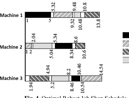
mare alike αp , βp. To illustratethe effects of the proposed robust JSS mathematical model, one can consider the Baker's example which was investigated earlier in this section. It is assumed that the maximum deviation for each processing time from the nominal value, tˆ, is equal to 10%. In other word, the true value,~ , takes tipm values in
[
0.9×tipm ,1.1×tipm]
. Furthermore suppose that: αp =λm =0.5 , βp =γm =0.8, ∀p,m. The robust optimum solution for this example is shown in Fig. 4.Fig. 4. Optimal Robust Job Shop Schedule
robustness level, but also it remains robust under the condition of heavier disruptions with a high probability. For more details see Bertsimas & Sim, 2004.
3. Proposed heuristic algorithm
Job shop scheduling problem is known NP-Hard in its classical type. Considering the number of used binary variables involved in a real-world problem formulation, we need to look for a near-optimal solution as an alternative using a heuristic approach. In the remaining part of this section, a heuristic algorithm based on the simulating annealing (SA) algorithm is proposed. SA is known to be one of the most successful algorithms amongst the other applied meta-heuristic ones and its acceptable performance is demonstrated by experience in the conducted researches relevant to scheduling problems, for example (Krishna, 1995), (Steinhofel, 1999), (Suresh, & Mohanasundaram, 2006), (Ponnambalam, 1999), (Bozejko, 2009).
The following algorithm is proposed to find a near-optimum schedule for the introduced robust JSS problem.
Sub Simulated annealing
k←1
Call Initial schedule generation
sbest← s
While k<K do
Call neighborhood Schedule generation (s)
If f(s´)≤f(s) or random[0, 1]<Paccept(s,s´,Tk) then
s ← s´.
Endif
If f(s´)<f(sbest) then
sbest← s´
Endif
k←k+1 Tk=α×Tk-1
Endwhile Endsub
Sub Initialschedule generation Do
Select one of the non-scheduled operations that it's all predecessors is already scheduled, randomly.
Compute the amount of protection function based on the desired robustness level, i.e. the required buffer times.
Compute the start and the completion time of the selected operation considering other scheduled operations in addition to the required buffer time.
If all operations are scheduled then Exit Do. Loop
Sub neighborhood Schedule generation (s)
Select one of the operations which are delayed in schedule s, e.g. opi.
Find the operation which causes the delay of opi in schedule s, e.g. opj.
Generate the schedule s´, by this new assumption that opi must be scheduled earlier than opj.
Note that all other operations must be scheduled in the same order of schedule s.
Endsub
In this part, s is a schedule, sbestis the best available solution, f(s) is the objective function value for
schedule s, k is the counter, K is the maximum iteration number which specifies the termination
criteria, Tk is the temperature in k-th iteration, α is the cooling factor which belongs to the interval (0,
1), and Paccept
(
s,s′,Tk)
is the probability function to accept non-improving solution s´, Eq. 16.
(
ss′Tk)
=Paccept , , (16)
Parameter tuning
In order to use the best combination of parameters defined in the proposed SA algorithm in this section, a full factorial design of experiment (DOE) approach is applied. As it is explained in the proposed algorithm, two parameters need to be tuned. These include T0 and α. In Table 2, three levels
for the parameters are considered, and therefore a 32 design is applied. The experiments contain 15
different instances randomly generated and solved by assuming each of 9 different combinations of (T0, α).
Table 2
Three levels of SA parameters
Level 1 Level 2 Level 3
α 0.97 0.98 0.99
T0 50 100 150
In order to compare the instances, the relative deviation index (RDI) is used. This index is obtained by
100, (17)
where, is the objective function value in the k-th instance. Mink and Maxk are the best and the
worst solutions obtained for each instance, respectively.
We have solved 15 different instances, each of which is associated with one of the combinations of (T0, α).
The results are analyzed by the means of analysis of variance (ANOVA) technique. The performed tests for analyzing the normality, homogeneity of variance and independence of residuals do not show any particular pattern in the experiments. Fig. 5 depicts the interaction plot for parameters T0 and α.
The combination of T0=150 and α=0.98 are calculated and produce better results compared to the
other evaluated combinations.
if f(s′)<f(s) 1
) ) ( ) ( (
exp
k
T s f s
f − ′
Fig 5. The achieved results for tuning the parameters of SA
The proposed SA algorithm is implemented in VB on a Laptop with Pentium IV Core 2 Duo 2.53 GHz CPU. The outputs of the algorithm are compared with optimum solutions achieved by Branch and Bound algorithm (B&B).
Each instance can be characterized by a number of parameters, such as number of jobs, number of machines, job routes, processing times, and the desired robustness parameters. The generated instances are based on the following assumptions:
• Processing times are all integer numbers between the interval [10, 20] generated at random.
• The objective is to minimize the total completion times of all jobs.
• The robustness parameters are set as follows: αp =λm=0.5 , βp =γm =0.8, ∀p,m. The outputs are shown in Table 3.
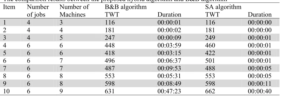
Table 3
The comparison results between the proposed hybrid algorithm and B&B algorithm Item Number
of jobs
Number of Machines
B&B algorithm SA algorithm
TWT Duration TWT Duration
1 4 3 116 00:00:01 116 00:00:00
2 4 4 181 00:00:02 181 00:00:00
3 4 5 247 00:00:09 249 00:00:01
4 6 6 448 00:03:59 460 00:00:01
5 6 6 418 00:03:15 422 00:00:01
6 6 7 496 00:06:37 501 00:00:01
7 6 7 487 00:09:53 488 00:00:05
8 6 8 553 00:05:31 553 00:00:05
9 6 8 598 00:08:49 598 00:00:11
10 6 9 631 00:47:23 662 00:00:40
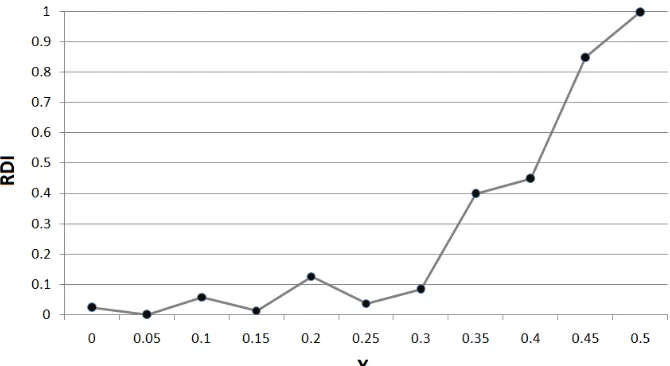
Fig 6. The achieved results for different interruption intervals
Fig. 6 shows that as the interruption intervals increases, in order to reach the same level of robustness, the TWT of the solutions are worsen.
4. Conclusion
We have presented a robust JSS problem which has the capability of handling the perturbation which exists amongst almost all input parameters. It is illustrated that, for many real world job scheduling problems, a small change in input parameters may lead us to some final solutions which are neither feasible nor optimal. The proposed method of this paper could guarantee that a small alteration in input parameters does not have any effect in the feasibility and the optimality of the robust one and does not alter from the crisp one. Besides, it is known that the common software packages are not able to find optimum solutions for real world application in a reasonable amount of time. Therefore, a SA algorithm has been proposed to find near optimal solutions in a reasonable amount of time. The effectiveness of the algorithm has been demonstrated, using some numerical examples and the results of SA have been compared with optimal solutions.
Acknowledgment
The author would like to thank the anonymous referees for their constructive comments on earlier version of this work.
References
Allet, S. (2003). Handling flexibility in a generalized job shop with a fuzzy approach. European Journal of Operational Research, 147, 312–333.
Baker, K. R. (1974). Introduction to sequencing and scheduling. New York: Wiley.
Ben-Tal, A., & Nemirovski, A. (2000). Robust solutions of linear programming problems contaminated with uncertain data. Mathematical Programming, 88, 411–424.
Bertsimas, D., & Sim., M. (2004). The price of robustness. Operations Research, 52, 35-53.
Bozejko, W., Pempera, J., & Smutnicki, C. (2009). Parallel Simulated Annealing for the Job Shop Scheduling Problem. In Proceedings of the 9th International Conference on Computational Science: Part I, 631 – 640.
Gharakhani, M., Taghipour, T. & Jalali Farahani, K. (2010). A robust multi-objective production planning, International Journal of Industrial Engineering Computations, 1(1), 73-78.
Garey, E.L., Johnson, D.S., & Sethi, R. (1976). The complexity of flowshop and job-shop scheduling. Mathematics of Operations Research, 1, 117–129.
Ginzburg, D.G., & Gonik, A. (2002). Optimal job-shop scheduling with random operations and cost objectives. International Journal of Production Economics, 76, 147–157.
Kacem, I., Hammadi, S., & Borne, P. (2002). Pareto-optimality Approach for Flexible Job-shop Scheduling Problems: Hybridization of Evolutionary Algorithms and Fuzzy Logic. Journal of Mathematics and Computers in Simulation, 60, 245-276.
Krishna, K., Ganeshan, K., & Janaki Ram D. (1995). Distributed Simulated Annealing Algorithms for Job Shop Scheduling, IEEE Transactions on systems. MAN. & Cybernetics, 25 (7), 1102-1109. Ponnambalam, S. G., Jawahar, N., & Aravindan, P. (1999). A simulated annealing algorithm for job
shop scheduling. Production Planning & Control, 10 (8), 767-777.
Shafia, M. A., Pourseyed Aghaee, M., Sadjadi, S. J., & Jamili, A. (2010). Robust Train Timetabling problem: Mathematical model and Branch and bound algorithm. Working paper
Shafia, M. A., Sadjadi, S. J., & Jamili, A. (2010). Robust Train Formation Planning. Proceedings of the IMechE Part F: Journal of Rail and rapid transit, 224(F2), 75-90.
Roghanian, E. & Foroughi, A. (2010). An empirical study of Iranian regional airports using robust data envelopment analysis, International Journal of Industrial Engineering Computations, 1(1), 65-72.
Soyster, A.L. (1973). Convex programming with set-inclusive constraints and applications to inexact linear programming. Operations Research, 21, 1154–1157.
Steinhofel, K., Albrecht, A., & Wong, C. K. (1999). Two simulated annealing-based heuristics for the job shop scheduling problem. European Journal of Operational Research, 118 (3) 524-548. Suresh, R.K. , & Mohanasundaram, K.M. (2006). Pareto archived simulated annealing for job shop