A b s t r a c t. Prediction of the influence of waste application on agricultural land and on the dynamics of infiltration is crucial for the optimum management of soil water as well as contaminants from runoffs. Three models (Philip’s, Kostiakov’s, and Horton’s) were investigated for their capability to describe water infiltration into a Typic Haplustult amended with different rates 10, 12.5, 25.0, 37.5 and 50.0 Mg ha-1of fresh (FW) and burnt (BW) rice-mill waste. Data were collected for two seasons between 1991 and 1992. Based on the values of the coefficient of correlation (R), the Kostiakov’s model provided the best fit with experimental data for both fresh (FW) and burnt (BW) rice-mill waste for the two seasons. It was followed by the Philip’s and then Horton’s models. However, transmissivity coefficients (A) of the Philip’s model were negative while Kostiakov’s coefficients were very insensitive to variations in application rates (q) of waste. Since the Horton’s coef-ficients indicated the highest sensitivity toq, these coef-ficients were expressed in terms ofqand then used for the prediction of cumulative infiltration. Variation in these coefficients withqwere exponential and parabolic with R2 ranging from 0.867 to 0.891 and 0.623 to 0.783 for the FW and BW amendments, respectively. Incorporation ofq in-creased R2from the poor negative average value of -0.382 to 0.748, thereby providing tools for advance prediction and analysis without actual waste application.
K e y w o r d s: infiltration, conditioned soils, models
INTRODUCTION
The need for safe waste disposal and improvement of soil characteristics often lead to waste application on agricultural land. Presence of waste on land alters hydro-dynamic chara-cteristics of soil-water movement as well as the
water availability to plants. Implications of wa-ste re-use on agricultural soil is not only im-portant for run-off management and leaching of contaminants to streams but also for the ge-neral water balance of the watershed.
One of the most important parameters con-trolling soil-water movement is infiltration. In-filtration varies both in time and space in re-sponse to soil variability, different management practices, climatic and hydrodynamic condi-tions [9]. Several models exist for describing infiltration of water into the soil [9,11-14]. Da-vidoff and Selim [6] investigated thecapability of eight models to describe water infiltration. Their results showed that Horton’s, Kostiakov’s and Philip’s equations provided best predic-tions over all the others values based on R2. Philip’s model was found better than, the Green and Ampt’s and a linearised form of the Philip’s equation was described by Swartzendruber and Youngs [17]. Philip’s two term equation has also been combined with the Kostiakov’s model equation to minimise the limitations of both models. For early and late stages of infiltration, the Kostiakov’s model was proved better than the Philip’s for examining effects of soyabean and crop rotation on infiltration. On the other hand, Horton’s, Philip’s, Green and Ampt’s, and Parlangi’s equations failed to adequately predict initial infiltration rates on the reclaimed surface of mined soils [5].
MODELLING INFILTRATION RATE IN CONDITIONED SOIL: COMPARISONS AND MODIFICATIONS
P.C. Nnabude1, J.C. Agunwamba2, J.S.C. Mbagwu3
1Department of Agricultural Engineering, Nnamdi Azikiwe University, P.M.B. 5025, Awka, Anambra State, Nigeria 2
Department of Civil Engineering, University of Nigeria, Nsukka, Nigeria
3
A technique for estimating parameters of the Philip’s equation has beendeveloped and tested on field data [3]. The technique provided information on the relationship between theA andKs parameters. The two term Philip equ-ation is inappropriate for a long term experi-ment because att®¥, infiltration rate equals saturated hydraulic conductivity of the soil (Ko). However,Amay be equal toKoand there is no general analytical relationship between the two [3]. Using the least squares may yield negative values of A [6]. Hence, infiltration rates predicted by the Philip’s equation when the parameters are determined by regression may be too low for the time period longer than duration of the experiment [15].
In the above research, an attempt was made to improve the models so that they could predict infiltration under different waste re-use and ma-nagement practices more accurately. Prediction under different waste re-use will equip the agri-cultural scientist or waste engineer with advanc-ed information on what to expect during waste application so that he could effectively manage or avoid any anticipated negative impact on the soil moisture and runoff characteristics. Hence, the research is aimed at improving the pre-dictive capabilities of the infiltration models under varying rates of fresh and burnt rice-mill waste.
MATERIALS AND METHODS
Experimental site
The research was conducted in Abakaliki agricultural zone of the south-eastern Nigeria. The area is situated at 8.°15’’ East longitude and 6.°30’’ North latitude. According to Agboola [1], local vegetation is transitional to the south-ern forest region and northsouth-ern semi-arid zone. Typically for the humid tropics, the area is characterised by high temperatures and high intensity rainfall. The climate is divided into definite dry and wet seasons. The wet season with mean annual rainfall of 1200-2000 mm runs from April to October while the dry season covers the rest of the year. The soil belongs to Ultisol category within Ezzamgbo soil
asso-ciation derived from shale parent material and classified as Typic Haplustult [8].
Field methods
The area was cleared, ploughed and harrowed in April 1991. The experimental plots were laid out in a randomised complete block design (RCBD) comprising eight treatments and control. Each experimental unit measured 3 m by 5 m and was replicated three times. The soil amendments consisted of two types of rice -mill waste namely - fresh (FW) and burnt (BW) waste. They were collected from the Abakaliki rice-mill factory and applied at the rates of 0.0, 12.5, 25.0, 37.5 and 50.0 Mg ha-1. The amen-dments were left to incubate for a period of two weeks before planting with maize. The influ-ence of these supplements were monitored in the following year to determine residual effects.
Laboratory methods
At the end of the first and second cropping seasons, bulk density, total and aeration poro-sities as well as organic carbon were determi-ned. Undisturbed core samples were used for the determination of bulk density, total and aeration porosity levels. Bulk density was deter-mined using the core method and the total po-rosity was calculated from the relationship between bulk density and particle density as follows:
Tp D
D b
p
= −
1 100
whereTp,Dband Dprepresent total porosity,
bulk density and particle density, respectively. Aeration porosity was calculated as:
Ap=Tp-Æv (0.1)
whereAprepresents aeration porosity andÆv
(0.1) represents percent volume of water con-tent at 0.1 bar suction.
Infiltration rate determination
The rate of water infiltration into the soil as influenced by the supplements was determined using a double ring infiltrometer method described by Bouwer [4]. In this method, double ring cylindrical metals with the diame- ters 30 and 40 cm for the inner and outer rings, respectively, were driven l0 cm deep into the soil of representative plots. Water was ponded at constant depth into two cylinders and the rate at which water moved into the soil was mea-sured. This was done at the end of the first and second cropping seasons.
Mathematical considerations
Infiltration data were into the Philip’s [14], Kostiakov’s [13] and Horton’s [11] models and analysed to estimate the parameters as follows:
Philip’s model:
f=1Sp t− +A
2
1
2 (1)
Kostiakov’s model:
f=K t1 −a (2)
Horton’s model:
f=fc+ (fo-fc) exp (-K2t) (3)
wheref- infiltration rate at timet;SpandA -sorptivity and transmissivity coefficients; K1
anda- model coefficients;foandfc- initial and final infiltration rates; K2- a constant
depen-ding primarily upon soil characteristics and vegetation.
The corresponding cumulative infiltration (I) are derived from the Eqs (1) and (3) using the relationship:
I= ∫otf fdt (4)
wheret- the final infiltration time.
RESULTS AND DISCUSSION
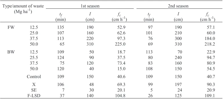
Cumulative infiltration (I) was generally higher with fresh (FW) than with burnt (BW) supplements for the corresponding amount of waste (Table l). There is a significant difference between their mean values at 5 % level. Table 2 shows variation of bulk density (p), total poro-sity (Tp), organic carbon (OC), and organic mat-ter (OM)with seasons and treatment (amount of waste).
Table 3 shows coefficients of correlation (R) and standard errors (s) of the Philip’s, Ko-stiakov’s and Horton’s models to the measured infiltration data for the 1st and 2nd seasons, respectively. Standard errors indicated a certain
Type/amount of waste (Mg ha-1)
1st season 2nd season
tf
(min)
I (cm)
fc
(cm h-1)
tf
(min)
I (cm)
fc
(cm h-1)
FW 12.5
25.0 37.5 50.0
135 107 113 65
190 160 220 310
52.9 62.6 97.3 225.0
97 101 76 69
190 210 300 310
57.1 60.0 184.0 218.2
BW 12.5
25.5 37.5 50.0
109 124 75 120
50 90 120 40
18.7 37.5 73.4 15.0
113 80 83 108
70 240 160 150
22.9 94.7 80.9 54.5
Control 109 150 40.6 109 150 40.7
X SE F-LSD
106 7 37
48 30 140
69.3 20.1 104.8
99 5 26
197 24 125
90.3 20.9 109.1 FW - fresh rice-mill waste, BW - burnt rice-mill waste,q- quantity and amount of waste.
T a b l e 1.Time to reach final infiltration rate, tf(min), cumulative infiltration (I), and final infiltration rate (fc) for each
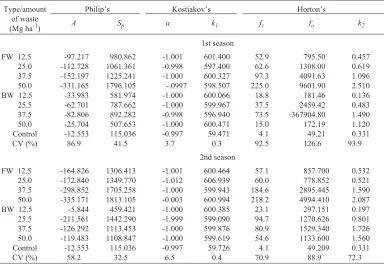
around scatter regression line [16]. Generally, the R values are high, indicating a good fit. The best fit was obtained with the Kostiakov’s model for all the data, followed by the Philip’s, and then the Horton’s.
The parameters of the models by Philip (A andSp), Kostiakov (aandk1) and Horton (fc,fo
andk2), determined by regression analysis are indicated in Table 4 for the seasons 1 and 2, re-spectively. The highest coefficients of variation
Type/ amount of waste (Mg ha-1)
r Tp OC OM
1st 2nd 1st 2nd 1st 2nd 1st 2nd
FW 12.5 25.0 37.5 50.0 1.60 166 1.47 1.58 1.58 1.61 1.58 1.53 36.7 37.4 44.4 40.7 40.2 38.6 40.3 42.4 1.76 2.43 3.23 3.55 1.76 2.39 2.51 3.11 3.03 4.20 5.57 6.12 3.03 4.13 4.33 5.37 BW 12.5 25.5 37.5 50.0 Control 1.67 1.65 1.62 1.51 1.77 1.70 1.57 1.45 1.63 1.72 37.7 37.6 39.0 43.2 33.1 35.7 40.8 45.4 38.5 35.1 2.39 2.59 3.15 3.15 1.51 2.20 1.76 2.20 3.35 1.60 4.13 4.47 5.43 5.15 2.99 3.78 3.03 3.78 4.06 2.78 X SE F-LSD 1.62 0.03 0.16 1.60 0.03 0.16 36.9 1.1 5.7 39.7 1.0 5.2 2.64 0.22 1.14 2.32 0.19 1.00 4.57 0.35 1.81 3.80 0.25 1.32
T a b l e 2.Variation in bulk density (r), total porosity (Tp), organic carbon (OC) and organic matter (OM) with amount of
waste (q) and season
Type/amount of waste (Mg ha-1)
Philip’s Kostiakov’s Horton’s
R S R S R S
1st season FW 12.5 25.0 37.5 50.0 BW 12.5 25.5 37.5 50.0 Control 0.996 0.935 0.997 0.996 0.990 0.997 1.000 0.999 0.989 2.822 7.008 2.544 6.364 1.224 1.582 0.149 0.621 1.224 1.000 0.999 0.998 1.000 1.000 1.000 1.000 0.999 1.000 0.002 0.151 0.021 0.004 0.004 0.001 0.003 0.018 0.004 0.966 0.949 0.923 0.956 0.999 0.854 0.947 0.994 0.992 0.264 0.443 0.414 0.275 0.042 0.958 0.3073 0.195 0.147 2nd season FW 12.5 25.0 37.5 50.0 BW 12.5 25.5 37.5 50.0 Control 0.988 0.989 0.996 0.999 0.821 0.992 1.995 0.993 0.989 14.994 17.537 6.337 3.985 17.220 30.667 3.198 7.470 1.224 1.000 0.999 1.000 1.000 1.000 1.000 1.000 0.999 1.000 0.001 0.026 0.006 0.005 0.003 0.005 0.005 0.017 0.004 0.961 0.985 0.985 0.807 0.992 0.984 0.915 0.952 0.992 0.391 0.247 0.115 0.651 0.193 0.081 0.382 0.536 0.147
were obtained for the Horton’s coefficients, indicating high sensitivity of fc, fo, and k to variations in the rate of application (q). Range of variations of the Kostiakov’s coefficients are very narrow: -0.997 to -1.005 (0.8%) foraand 596.940 - 601.400 (0.8%) forK1whileqvaries
from 12.5 to 50 Mg ha-1(300%).
Generally speaking, lower model coef-ficients were obtained from BW than from FW which corroborated the occurrance of higher
infiltration capacity in the latter. There is a si-gnificant difference (P < 0.05) in mean values of the coefficients obtained for the soil treated with FW and BW except for the Kostiakov’s coefficients andfo(Table 5). This again shows insensitivity of the Kostiakov’s coefficients to different applications. The valuefo= 367904.8 in Table 4 for BW = 37.5 Mg ha-1was not used in all calculations because it was too high (accounting for 98 % ofSfo), about 100 orders
Type/amount of waste (Mg ha-1)
Philip’s Kostiakov’s Horton’s
A Sp a k1 fc fo k2
1st season FW 12.5 25.0 37.5 50.0 BW 12.5 25.5 37.5 50.0 Control CV (%) -97.217 -112.728 -152.197 -331.165 -33.983 -62.701 -82.806 -25.704 -12.553 86.9 980.862 1061.361 1225.241 1796.105 581.974 787.662 892.282 507.653 115.036 41.5 -1.001 -0.998 -1.000 -.0997 -1.000 -1.000 -0.998 -1.000 -0.997 3.7 601.400 597.400 600.327 598.507 600.066 599.967 596.940 600.471 59.471 0.3 52.9 62.6 97.3 225.0 18.8 37.5 73.5 15.0 4.1 92.5 795.50 1308.00 4091.63 9601.90 181.46 2459.42 367904.80 172.19 49.21 126.6 0.457 0.619 1.096 2.510 0.136 0.483 1.490 1.120 0.331 93.9 2nd season FW 12.5 25.0 37.5 50.0 BW 12.5 25.5 37.5 50.0 Control CV (%) -164.826 -172.840 -298.852 -335.171 -5.844 -211.561 -126.292 -119.483 -12.553 58.2 1306.413 1349.770 1705.258 1813.105 459.421 1442.290 1113.453 1108.847 115.036 32.5 -1.001 -1.012 -1.000 -0.003 -1.000 -1.999 -1.000 -1.000 -0.997 6.5 600.464 606.939 599.943 600.994 600.385 599.090 599.876 599.619 59.726 0.4 57.1 60.0 184.6 218.2 23.1 94.7 80.9 54.6 4.1 70.9 857.700 778.852 2895.445 4994.410 297.151 1270.626 1529.340 1133.600 49.209 88.9 0.532 0.521 1.590 2.087 0.197 0.801 1.726 1.560 0.331 72.3
T a b l e 4.Parameters of various models determined by regression analysis for the first (1991) and second (1992) seasons
Type of waste
A Sp a K1 fc fo K2
FW x d BW x d Difference of means -208.125 97.950 -83.547 67.384 Si 1404.764 327.922 861.698 345.044 Si -1.002 0.0046 -1.000 0.0074 N Si 600.747 2.827 599.551 1.142 N Si 119.713 76.260 49.753 30.720 Si 3165.430 3065.757 1006.300 851.489 N Si 1.177 0.798 0.564 0.557 Si
greater than expected. If this value is used, there will be a significant difference in the mean values offo. Variations of the coefficients withq are shown in Table 4.AlthoughAandSpvary,
the negative values of A obtained has no physicalsignificance. It is noteworthy that such negative values have also been reported in many infiltration studies [5,7,15,18]. Besides,Aand Sp are not as sensitive as the Horton’s coefficient. Hence, in this research, the Hor-ton’s coefficients are used for the incorporation ofqin the prediction of cumulative infiltration. Hence, only the graphs of the results of the Hor-ton’s equation are shown in Fig. 1a, even though it gave poor predictions (R2= -0.170 and -0.677 for the 1st and 2nd seasons, respectively) as well. These results clearly indicate unsuc-cessful prediction ofIon the plots treated with
waste without any modifications such as incor-porating the effects ofq. For the above reasons the Horton’s coefficients, were expressed in terms ofq.
Since the curves for the two seasons are similar, data is pooled together. A marked dif-ference between the values from FW and BW (Table 5), shows that the relationship between each of the coefficients and q is a straight line/exponential and parabolic for FW and BW, respectively. Using the data from Table 4, the following equations were obtained:
- for FW:
fo= 315 exp 0.061w; R2= 0.882,
S= 0.689 (5)
fc= 29 exp 0.04w; R2= 0.867,
S= 0.259 (6)
0 100
100
200 200
Measured infiltration (cm)
Modeled
infiltration
(cm)
300 300
400 400
SEASON 2
Measured infiltration (cm)
0 100
100
200 200
Modeled
infiltration
(cm)
300 300
400 400
SEASON 2
0 100
100
200 200
Measured infiltration (cm)
Modeled
infiltration
(cm)
300 300
400 400
SEASON 1
0 100
100
200 200
Measured infiltration (cm)
Modeled
infiltration
(cm)
300 300
400 400
SEASON 1
Fig. 1.Measured vs. model cumulative infiltration from the unmodififed (a) and modified (b) Horton’s infiltration model for seasons 1 and 2.
a
K2= 0.05w- 0.39; R2= 0.891,
S= 0.593 (7)
- for BW:
fo= -2466.06 + 273.34w- 4.24w2; R2= 0.697,
S= 16.325 (8)
fc= -72.89 + 9.18w- 0.14w2; R2= 0.623,
S= 3.40 (9)
K= -1.236 + 0.132w-0.002w2; R2= 0.783,
S= 0.315. (10)
Predictions of Ibased on these equations are shown in Fig. 1. The equations that fit the predicted values for the 1st and 2nd seasons are respectively:
Imodel= 0.735Imeasured+ 67.088; R2= 0.782;
S = 38.506 (11)
Imodel= 0.845Imeasured- 0.422; R2= 0.714;
S= 40.350 (12)
which is a great improvement over the predic-tions from the control coefficients. An ex-pression of this nature could be helpful in an advanced analysis of the impact of land ap-plications of different types and quantities of waste. Several alternatives could be investi-gated to arrive at the optimum waste re-use with respect to minimum contaminant release in runoffs and available moisture for plant growth.
CONCLUSION
The paper considered a model incorporating fresh (FW) and burnt (BW) agro-waste applica-tion rate (q) for an advanced prediction of cumu-lative infiltration without actual measurements on the treated site. While the Kostiakov’s model gave the best fit for the infiltration data, its coefficients were very insensitive to the variations inq. The Philip’s coefficients were more sensitive than the Kostiakov’s but had unrealistic negative
transmi-ssivity coefficients. Coefficients of the Horton’s model were very sensitive and found to be expo-nentially/linearly and parabolically related to q with R2ranging from 0.882 to 0.891 in FW and 0.623 to 0.783 in BW. Such models could be useful for advanced analyses and prediction of different waste re-use impacts on runoff and infiltration without actual application of the waste which could be expensive.
ACKNOWLEDGMENT
The project was carried out with the financial assistance provided by the African Academy of Sciences (AAS) under the Capa-city Building in Soil and Water Management (SWM).
REFERENCES
1. Agboola S.A.: An Agricultural Atlas of Nigeria. Oxford University Press, 43-48, 1979.
2. Allison F.E.:Soil Organic Matter and Its Role in Crop Production. Elsevier Scientific, New York, 1973. 3. Bach L.B., Wierenga P.J., Ward T.J.: Estimation of
the Philip infiltration parameters from rainful simula-tion data. Soil Sci. Soc. Am. J., 50, 1319-1323, 1982. 4. Bouwer H.:Intake Rate: Cylinder Infiltrometer. In: Methods of soil analysis. (Ed. Klute A.) Part I: Physical and Mineralogical Methods. 2nd Edition, 825 ASA, m SSSA Madison Wisconsin, U.S.A., 1986.
5. Cook D.F., Magnett W.L., Jones J.N., Shanholtz V.O., Hockman E.L.: Evaluation of infiltration equations on reclaimed mined soils. ASAE Paper SER 83-007. Am. Soc. Agric. Engrs., 5t. Joseph, MI, 1982. 6. Davidoff B. Selim H.M.:Goodness of fit for eight
water infiltration models. Soil Sci. Soc. Am. J., 50, 759-764, 1986.
7. Fahad A.A., Mielke L.N., Flowerday A.D., Swart-zendruber D.:Soil physical properties as affected by soyabeans and other cropping sequences. Soil Sci. Soc. Am. J., 46, 377-381, 1982.
8. FDALR: Reconnaissance soil survey of Anambra State, Nigeria. Soils Report. FDALR Kaduna, 1985. 9. Green W.H., Ampt G.A.:Studies on soil physics: I.
The flow of air and water through soils. J. Agric. Sci., 4, 1-24, 1911.
10.Gumps F.A., Workentin B.P.:The effect of bulk density and initial water content on intiltration in dry soil samples. Soil Sci. Soc. Am. Proc., 36, 720-724, 1972.
11. Horton R.E.:Approach toward a physical interpre-tation of infiltration capacity, Soil Sci. Soc. Am. Proc., 5, 399-417, 1940.
13.Kostiakov A.N.:On the dynamics of the coefficient of water-percolation in soils and on the necessity for studying it from a dynamic point of view for purpose of amelioration. Trans Int. Congr. Soil Sci., 17-21, 1932. 14.Philip J.R.:Theory of infiltration. Adv. Hydrosci., 5,
215-296, 1969.
15.Skaggs R.W., Huggins L.E., Monke E.J., Foster G.R.: Experimental evaluation of infiltration equa-tions. Trans. ASAE, 822-828, 1969.
16.Spiegel M.R.: Theory and Problems of Statistics. Shaum’s Outline Series. McGraw-Hill Metric Editions, McGraw-Hill. Book Co., New York, 1987.
17.Swartzendruber D., Youngs E.G.:A comparison of physically-based infiltration equations: Soil Sci., 117, 165-167, 1974.