MAPPING ACTIVITY DIAGRAM TO PETRI NET:
APPLICATION OF MARKOV THEORY FOR
ANALYZING NON-FUNCTIONAL
PARAMETERS
H. Motameni*
Department of Computer Engineering, Islamic Azad University Science and Research Branch, Tehran, Iran
A. Movaghar
Department of Computer Engineering, Sharif University of Technology Tehran, Iran
M. Fadavi Amiri
Department of Computer Engineering, Iran University of Science and Technology Tehran, Iran
*Corresponding Author
(Received: January 17, 2006 – Accepted in Revised Form: March 18, 2007)
Abstract The quality of an architectural design of a software system has a great influence on achieving non-functional requirements of a system. A regular software development project is often influenced by non-functional factors such as the customers' expectations about the performance and reliability of the software as well as the reduction of underlying risks. The evaluation of non-functional parameters of a software system at the early stages of design and its development process are often considered as major factors in dealing with these issues. Because these evaluations can help us to choose the most proper model which is the securest and the most reliable.In this paper, a method is presented to obtain performance parameters from Generalized Stochastic Petri Net (GSPN) to be able to analyze the stochastic behavior of the system. The embedded Continuous Time Markov Chain (CTMC) is derived from the GSPN and the Markov chain theory is used to obtain the performance parameters.
Keywords UML, Activity Diagram (AD), Generalized Stochastic Petri Net (GSPN), Continuous Time Markov Chain (CTMC), Non-Functional Parameters, Markov Reward Models
ﻩﺪﻴﻜﭼ
ﻴﺳﮏﻳﯼﺭﺎﻤﻌﻣﯽﺣﺍﺮﻃﺖﻴﻔﻴﮐ ﯼﺭﺍﺰﻓﺍﻡﺮﻧﻢﺘﺴ
ﯽﺗﺎﻴﻠﻤﻋﺮﻴﻏﯼﺎﻫﺯﺎﻴﻧﻥﺩﺭﻭﺁﺖﺳﺪﺑﺭﺩﯼﺩﺎﻳﺯﺮﻴﺛﺎﺗ ﺩﺭﺍﺩ
.
ﺮﻴﻏﯼﺎﻫﺭﻮﺘﮐﺎﻓﻪﻠﻴﺳﻭﻪﺑﺐﻠﻏﺍﻪﻌﺳﻮﺗﻝﺎﺣﺭﺩﯼﺭﺍﺰﻓﺍﻡﺮﻧﻩﮊﻭﺮﭘﮏﻳ ﯽﻳﺍﺭﺎﮐﻩﺭﺎﺑﺭﺩﯼﺮﺘﺸﻣﺕﺍﺭﺎﻈﺘﻧﺍﺪﻨﻧﺎﻣﯽﺗﺎﻴﻠﻤﻋ
ﺩﺎﻤﺘﻋﺍﺖﻴﻠﺑﺎﻗﻭ ﯽﻣﺶﻫﺎﮐﻥﺁﯽﺳﺎﺳﺍﯼﺎﻫﮏﺴﻳﺭ،ﻪﺘﻓﺮﮔﺭﺍﺮﻗﺮﻴﺛﺎﺗﺖﺤﺗ
ﺎﻳ ﺪﺑ . ﮏﻳﯽﺗﺎﻴﻠﻤﻋﺮﻴﻏﯼﺎﻫﺮﺘﻣﺍﺭﺎﭘﯽﺑﺎﻳﺯﺭﺍ
ﺭﺩﺚﺤﺑﻦﻳﺍﯽﺳﺎﺳﺍﯼﺎﻫﺭﻮﺘﮐﺎﻓﺕﺭﻮﺻﻪﺑﺐﻠﻏﺍ،ﻥﺁﻪﻌﺳﻮﺗﺪﻨﻳﺍﺮﻓﻭﯽﺣﺍﺮﻃﻪﻴﻟﻭﺍﻞﺣﺍﺮﻣﺭﺩﯼﺭﺍﺰﻓﺍﻡﺮﻧﻢﺘﺴﻴﺳ ﯽﻣﻪﺘﻓﺮﮔﺮﻈﻧ ﯽﻣﺎﻫﯽﺑﺎﻳﺯﺭﺍﻦﻳﺍﻭﺪﻧﻮﺷ
ﺪﻨﻨﮐﮏﻤﮐﻝﺪﻣﻦﻳﺮﺗﻦﺌﻤﻄﻣﻭﻦﻳﺮﺗﻦﻣﺍﺏﺎﺨﺘﻧﺍﺭﺩﺪﻨﻧﺍﻮﺗ .
،ﻪﻟﺎﻘﻣﻦﻳﺍﺭﺩ
ﺖﺳﺩﻪﺑﯼﺍﺮﺑﯽﺷﻭﺭ ﺯﺍﺎﻫﺮﺘﻣﺍﺭﺎﭘﻦﻳﺍﻥﺩﺭﻭﺁ
" ﯽﻣﻮﻤﻋﯽﻓﺩﺎﺼﺗﯼﺮﺘﭘﻪﮑﺒﺷ "
(GSPN) ﯽﻣﯽﻓﺮﻌﻣ ﺩﻮﺷ ﺭﺎﺘﻓﺭﻥﺍﻮﺘﺑﺎﺗ
ﺍﺭﻢﺘﺴﻴﺳﯽﻓﺩﺎﺼﺗ ﺗ
ﻞﻴﻠﺤ ﺩﻮﻤﻧ . ﺯﺍﻪﺘﺳﻮﻴﭘﻥﺎﻣﺯﻑﻮﮐﺭﺎﻣﻩﺮﻴﺠﻧﺯﺲﭙﺳ GSPN
ﯼﺍﺮﺑﻑﻮﮐﺭﺎﻣﯼﺭﻮﺌﺗﻭﻩﺪﺷﻖﺘﺸﻣ
ﯽﻣﺭﺍﺮﻗﻩﺩﺎﻔﺘﺳﺍﺩﺭﻮﻣﺎﻫﺮﺘﻣﺍﺭﺎﭘﻦﻳﺍﻥﺩﺭﻭﺁﺖﺳﺩﻪﺑ ﺩﺮﻴﮔ
.
1. INTRODUCTION
A PN is an abstract, formal model of information
systems, particularly systems that may exhibit asynchronous and concurrent activities. The major use of PNs has been the modeling of systems of events in which it is possible for some events to occur concurrently but there are constraints on the concurrence, precedence, or frequency of these occurrences.
There are three general characteristics of PNs that make them interesting in capturing concurrent, object-oriented behavioral specifications. First, PNs allow the modeling of concurrency, synchronization, and resource sharing behavior of a system. Secondly, there are many theoretical results associated with PNs for the analysis of such issues as deadlock detection and performance analysis. Finally, the integration of PNs with object oriented software design architecture could provide a means for automating behavioral analysis [1].
We present a method for obtaining non-functional parameters from GSPN. The reason for using GSPN is that, there are some methods for transforming UML diagrams to GSPN as an example one of them is introduced in [2,3].
Currently the Unified Model Language (UML) diagrams are widely used in the field of software design as it is easy to use in comparison to other alternatives, and is powerful in describing different aspects of a system. However, the semi-formal properties of the UML diagram cannot satisfy the industry's need in predicting the non-functional parameters of the software in the early stages of the software life cycle.
Since it is not possible to use UML diagrams for performance evaluation, they were translated to Generalized Stochastic Petri Net (GSPN) [2,3], a more formal model that enables the authors to do the performance evaluations.
The authors' previous work on AD includes the transformation of AD to Colored Petri Net [3, 4], where some performance measures could be obtained using simulation. The simulation-based measurements seem to be more straightforward compared to its alternatives, which are analytic methods.
First a brief discussion on GSPN is presented, then UML will be disscussed to introduce its fundamentals and history.
For the next step transforming AD to LGSPN(GSPN) is discussed and then how a
CTMC is derived from GSPN. Finally, performance evaluation on the derived CTMC is conducted and a case study is explained.
In this research, analytic methods are used to obtain results that are more accurate. Although using these kinds of methods induces some computational complexities to the calculation of system performance, the gained results are more reliable compared to simulation techniques. Therefore, analytic methods remain as the only choice for evaluating critical systems, but we should consider that this method is more useful in small systems because it is possible to have more details
2. RELATED WORK
The Use of Stochastic Petri Net (SPN) and its extensions have been discussed in several papers [2,5,6,7 and 8]. Merseguer et al. used the derived SPN from the UML model to evaluate performance of internet based software retrieval systems [7]. Derivation of an executable GSPN model from a description of a system expressing a set of UML State Machines (SMs) was reported in [9].
A group of works is devoted to transforming the software model to Colored Petri Net (CPN), which seems to be more related to software properties than the other UML extensions [10-15].
In the authors' previous works [4,16], the UML model was transformed to CPN and then analyzed by means of simulation. Trowitzsch et al. have transformed the software UML diagrams to SPN models for performance evaluation of real-time systems [5].
Most of the previous works discussed transforming the software model to analytical models or evaluating the performance model. In other words, none of them provides an integrated method, which can start from software models and terminate with some derived performance parameters.
software model to GSPN some performance parameters are calculated. In this paper, the performance model is evaluted in a way that leads to gain meaningful parameters of the system like reliability and security.
3. REVIEWING THE GSPN AND UML
3.1. GSPN
The basic PN model includes two components: places and transitions connected together via arcs to model system behavior; however, it may be extended by introducing the notion of time, leading to timed Petri nets (TPN) for a performance analysis of Petri Nets quantitative analysis. In TPN an exact time is associated to each transition. A timed PN is called a SPN, when random variables are used in specifying the time behavior. Whereas, it has been shown that SPNs are, under certain conditions, isomorphic to homogeneous Markov chains, by analyzing metrics of the Markov chain (such as the steady state probability distribution) it is possible to investigate the behavior of the underlying system being modeled by the PN [20].GSPN is defined as a PN N = (P,T,W,M0) with
its transition set T divided into two sub-sets TI and
TT, defining respectively the set of immediate and
timed transitions. Immediate transitions are fired immediately once they are enabled, whereas, timed transitions are fired after a random, exponentially distributed, enabling time. Hence, in GSPN N, transitions t ∈ TT are associated with a (possibly
marking-dependent) firing rate, r(t) that constitutes the defining parameter of the corresponding exponential distribution.
The above characterization of immediate and timed transitions implies that in a net reachable marking, m, where, both, immediate and timed transitions are enabled, immediate transitions have precedence over the timed ones (since they are instantaneous). Furthermore, in such a marking m has zero duration in the net dynamics, and therefore, it is characterized as vanishing. On the other hand, a marking m in which all enabled transitions are timed transitions and has zero duration; therefore, such a marking is characterized as tangible.
Given a marking m with a set of
simultaneously enabled immediate transitions, I(m), the modeler must provide a probability distribution regulating the firing of the transitions in I(m). In the GSPN terminology, this probability distribution is characterized as a random switch E = {W1, W2, ...,
W(m)}. Furthermore, if a set of random switches
regulating the net behavior are marking-dependent, they are characterized as dynamic; otherwise, they are static [21].
3.2. UML
UML consists of a set of graphs orcharts with explanatory comments that can be expressed either in a formal way or in natural language. Each diagram has a specific and precise position in the design process. An activity diagram is a dynamic diagram that shows the activity and the event that causes the object to be in the particular state. The activity is triggered by one or more events, and it may result in one or more events that may trigger other activities or processes. The biggest disadvantage of activity diagrams is that they do not clearly explain which objects execute which activities, and the way that the contection works between them. However, labeling of each activity with the responsible object can be performed. Often it is useful to draw an activity diagram early in the modeling of a process, to help understand the overall process [22].
3.2.1. Annotating AD
Additional information4. TRANSFORMING AD TO LGSPN
The transformation algorithm used to translate the activity diagram to the GSPN model is the one that is explained by Merseguer et al [2]. As long as the provided formalism seems to be well formed and well described, it was preferred to be used in this research to define an alternative. The only change made to the use of the algorithm is to relate the ratios (like security, dependability etc) assigned to the UML AD to GSPN elements. These ratios are then included in the LGSPN together with firing rates of transitions and the weights of immediate transitions.
The parameters like security ratio and reliability ratio of the action are just attached to those AD transitions that represent an action. These parameters are then simply related to time transitions of the LGSPN, which the tags are attached to. The parameters attached to the action states are attached to all of the places existing in the transformation of that element to LGSPN. Once the GSPN system is defined, some structural properties may be computed to perform a validation of the model. First, P and T semi-flows can be computed to check whether the net is structurally bounded and whether it may have home-states. Other structural results that may be computed are the Effective Conflict Sets (ECSs) of the model. These results ensure that the net is suitable for a numerical evaluation yielding the steady-state probabilities of all its markings [3].
5. DERIVING THE EMBEDDED CTMC
The stochastic process associated with k-bounded GSPN systems with M0, as their home state, can be
classified as a finite state space, stationary (homogeneous), irreducible, and continuous-time semi-Markov process [3]. In the case of GSPNs, the Embedded Markov Chain (EMC) can be recognized as disregarding the concept of time and focusing attention on the set of states of the semi-Markov process.
The specifications of a GSPN system are sufficient for the computation of the transition probabilities of such a chain. The CTMC associated with a given GSPN (the term GSPN is used instead of LGSPN, as the labels provided by
the LGSPN do not have any effect on analyzing of the net) system is obtained by applying some simple rules:
The CTMC state space S = {si} corresponds to
the reachability set RS(M0) of the PN associated
with the GSPN (Mi ↔ si).
The transition rate from state si (corresponding
to marking Mi) to state sj (Mj) is obtained as the
sum of the firing rates (for timed transitions) or weights (for immediate transitions) of the transitions that are enabled in Mi and whose firings
generate marking Mj.
Based on the simple rules listed above, it is possible to devise algorithms for the automatic construction of the infinitesimal generator (also called the state transition rate matrix) of the isomorphic CTMC, starting from the GSPN description. Denoting this matrix by U, with wk the
firing rate (or weight for immediate transitions) of Tk
and with Ej(Mi) = {h : Th∈ E(Mi)∧ Mi | Th > Mj} the
set of transitions whose firings bring the net from marking Mi to marking Mj, the components of the
transition probability matrix would be:
i q
k W ) i M ( j E k T j , i U
∑ ∈
= (1)
Let RS, TRS and VRS indicate the reachability set, tangible reachability set and vanishing reachability set of the stochastic process the following relation is true among these sets:
φ = ∩ ∪
= TRS VRSandVRS TRS
RS (2)
By ordering the markings so that the vanishing ones correspond to the first entries of the matrix and the tangible ones to the last, the transition probability matrix U can be decomposed in the following manner:[3]
⎥ ⎦ ⎤ ⎢ ⎣ ⎡ + ⎥ ⎦ ⎤ ⎢ ⎣ ⎡ = + =
F E
0 0 0 0
D C B A
U (3)
6. ANALYZING THE DERIVED CTMC
⎩ ⎨ ⎧ = ψ ψ = ψ 1 T 1 U (4)
in which ψ is a row vector representing the steady-state probability distribution of the EMC, can be interpreted in terms of numbers of state-transitions performed by the EMC. Indeed, 1/ψi is the mean
recurrence time for state si (marking Mi) measured
in number of transition firings.
Although this method is computationally acceptable when the number of vanishing states are small (compared with the number of tangible states) but it also computes the probability of vanishing markings that does not increase the information content of the final solution since the time spent in these markings is known to be null. Moreover, vanishing markings, created by enlarging the size of the transition probability matrix U, tend to make the computation of the solution more expensive and in some cases even impossible to obtain. So the model must be reduced by computing the total transition probabilities among tangible markings only, thus identifying a Reduced EMC (REMC). The transition probability matrix of the REMC can thus be expressed as:[3]
H E F
U′= + (5)
Where
[
]
⎪⎩ ⎪ ⎨ ⎧ − − ∑ = = D 1 C I 0 n 0 k Ck)D (H (6)
The solution of the problem
⎩ ⎨ ⎧ = ψ′ ′ ψ′ = ψ′ 1 T 1 U (7)
gives ψ a row vector representing the steady-state probability distribution of the REMC. The infinitesimal generator q´ of the CTMC associated with a GSPN can be constructed from the transition probability rate matrix U´ of the REMC by dividing each of its rows by the mean sojourn time (1/ui) of the corresponding tangible marking
(The sojourn time is the time spent by the PN
system in a given marking M). To conform to the standard definition of the infinitesimal generators, the diagonal elements of Q´ are set equal to the negative sum of the off diagonal components:
⎪ ⎪ ⎩ ⎪⎪ ⎨ ⎧ = ∑ ≠ ′ − ≠ ′ = ′ j i i j ij
q j i j i u i J S 1 j i
q (8)
An alternative way of computing the steady-state probability distribution over the tangible markings is thus that of solving the following system of linear matrix equations:
⎩ ⎨ ⎧ = η = ′ η 1 T 1 0 Q (9)
The probability that a given transition Tk ∈ E(Mi)
fires first in marking Mi has the expression:
i q / k W } i M | k T {
P = ′ (10)
Using the same argument, it can be observed that the average sojourn time in marking Mi is given by
the following expression:
i q / 1 i J
S = ′ (11)
The steady-state distribution η´ is the basis for a quantitative evaluation of the behavior of the SPN that is expressed in terms of performance indices. These results can be computed using a unifying approach in which proper index functions (also called reward functions) are defined over the markings of the SPN and an average reward is derived using the steady-state probability distribution of the SPN. Assuming that r(M) represents one of such reward functions, the average reward can be computed using the following weighted sum:
∑ ∈ η = ) 0 M ( RS i
M r(Mi) i
R (12)
• The probability of a particular condition of the GSPN: Assuming that condition Y(M) is true only in certain markings of the PN. Reward Function can be defined as follows [3]:
⎩ ⎨ ⎧ = = otherwise 0 true ) M ( Y 1 ) M (
r (13)
The desired probability P{Υ} is then computed using the equation. The same result can also be expressed as: ∑ ∈ η′ = A i M i } Y {
P (14)
where
A = {Mi∈ RS (M0) : Υ (Mi) = true}.
• The expected value of the number of tokens in a given place: In this case, the reward function r(M) is simply the value of the marking of that place (say place j):
n ) i P ( M if n ) M (
r = = (15)
Again, this is an equivalent to identify the subset A(j, n) of RS(M0) for which the number of tokens in
place pj is n (A(j,n) = {Mi | RS(M0) ∈ Mi(pj) = n})
the expected value of the number of tokens in pj is
given by:
{
}
∑ > = 0 n ] ) n ,j ( A P n [ ] ) j p ( M [E (16)
where the sum is obviously limited to values of n ≤ k, if the place is k bounded.
• The mean number of firings per unit of the time of a given transition: Assume that the firing frequency of transition Tj (the throughput of Tj)
was wanted to computed; observing that a transition may fire only when it is enabled, the reward function assumes the value wj in every
marking that enables Tj :
⎩ ⎨ ⎧ ∈ = otherwise 0 ) M ( E j T j W ) M (
r (17)
The same quantity can also be computed using the more traditional approach of identifying the subset Aj of RS(M0) in which a given transition Tj is
enabled (Aj = {Mi∈ RS(M0) : Tj ∈ E (Mi)}). The
mean number of firings of Tj per unit of time is
then given by:[3]
∑ ∈ η = j A i
M j i
W i
f (18)
As we know, Petri nets are not only used as a formalism for describing the behavior of distributed/parallel systems and for assessing their qualitative properties, but also as a tool for computing performance indices that allow the efficiency of these systems to be evaluated. As these basic parameters are computed, some more meaningful information can be derived. For example, a metric formula comparing the security of different architectures can be gained by using the equation: ∑ ∈ ∗ ∑ ∈ ∑ ∈ + ∑ ∈ ∗ = P
p Sp Tp)/ p PSJp))/2 (
T t ft T
t St ft)/ ((
. Net Security
(19) Where St is the data security factor associated to
the transition t, ft is the firing rate of t, Sp the data
security factor associated to the place p, Tp is the
expected time in which there is a token in place p. This is similar to the authors' previous work using simulation. Identically the reliability can be computed, but because the reliability is usually related to the processes of the system, the reliability factor is just usually associated to the transitions than the places:
⎟ ⎠ ⎞ ⎜ ⎝ ⎛∑ ∈ ∗ ∑ ∈ = T t ft T
t RLt ft)/ .
Net liability Re
7. CASE STUDY
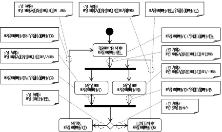
Figure 1 shows the activity diagram of a parallel system. The system operations are modelled as follows. A set of new data is read (firing of transition tnew), and two processes are started in
parallel with the same set of data (the fork operation-firing of tstart). When both processes are
complete (firing of tpar, and tpar1, respectively), a
synchronization takes place (the join operation-firing of transition tsyn). The consistency of the two
results is then controlled, and one of the two transitions tOK or tKO fires, indicating whether the
results are acceptable, or not. If the results are not consistent, the whole computation is repeated on the same data, after a further control (firing of
«PAStep»
{PArespTime='assm',max(N,'s')} {PArespTime='assm',max(Teta,'s')} «PAStep» {Security=0.69 , Reliability=0.92}
«PAStep» {PAprob=0.99} {Security=0.85 , Reliability=0.73} «PAStep»
{PArespTime='assm',max(M1,'s')} {Security=0.63 , Reliability=0.83}
{Security=0.8 , Reliability=0.6} «PAStep»
{PArespTime='assm',max(M2,'s')} «PAStep»
{PArespTime='assm',max(L,'s')} {Security=0.7 , Reliability=0.95}
«PAStep» {PAprob=0.01} Do Part2
{Security=0.7}
Do I/O {Security=0.78}
Check Data {Security=0.83} Do Part1
{Security=0.56} Input New Data
{Security=0.69}
Figure 1. Activity diagram that specifies a parallel system.
t
newt
startt
synt
part
par1t
KOt
OKt
I/Ot
check2
1 3
4 5
6 7
8
9
TABLE 1. Timed Transitions of Figure 2 and Their Specifications.
Transition Rate Semantics
Tnewdata λ Infinite-server
Tpar1 μ1 Single-server
Tpar2 μ2 Single-server
TI/O ν Single-server
Tcheck θ Single-server
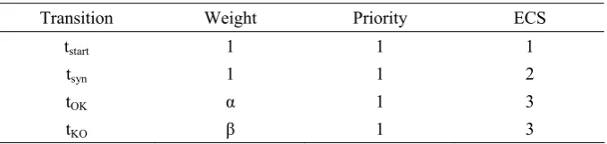
TABLE 2. Immediate Transitions of Figure 2 and Their Specifications.
Transition
Weight Priority ECS
tstart 1 1 1
tsyn 1 1 2
tOK α 1 3
tKO β 1 3
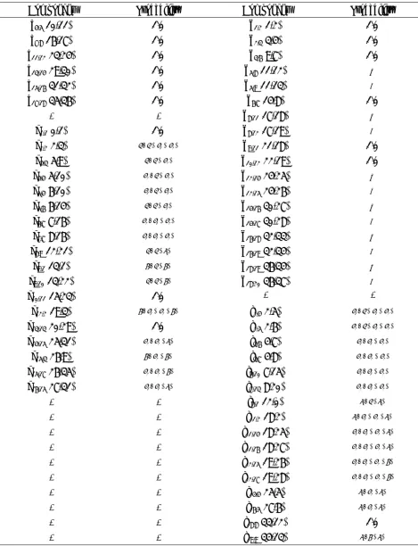
TABLE 3. The Markings of the GSPN Presented in Figure 2.
M0 = 2p1 M1 = p1 + p2 M2 = p1 + p3 + p4 M3 = p2 + p3 + p4 M4 = 2p3 + 2p4 M5 = p1 + p4 + p5 M6 = p1 + p3 + p6 M7 = p3 + 2p4 + p5 M8 = 2p3 + p4 + p6 M9 = p2 + p4 + p5 M10 = P1+p5+p6 M11 = p1 + p7
M12 = p1 + p9 M13 = p1 + p8 M14 = p2 + p3 + p6 M15 = 2p4 + 2p5 M16 = p3 + p4 + p5 + p6 M17 = p3 + p4 + p7 M18 = p3 + p4 + p9 M19 = p3 + p4 + p8 M20 = 2p3 + 2p6 M21 = p2 + p9 M22 = p2 + p8 M23 = p4 + 2p5 + p6 M24 = p4 + p5 + p7 M25 = p3 + p5 + 2p6 M26 = p4 + p5 + p8 M27 = p3 + p6 + p9 M28 = p3 + p6 + p8 M29 = p3 + p5 + 2p6 M30 = p3 + p6 + p7 M31 = p5 + p6 + p7 M32 = p7 + p9 M33 = 2p9 M34 = p8 + p9 M35 = p5 + p6 + p8
M36 = p7 + p8 M37 = 2p8
tcheck); otherwise, the results are output (firing of
transition tI/O), and a new set of data is considered.
The model is then converted to a GSPN model by the methodology [2]. The conversion result is shown in Figure 2. The model specifications are shown in Tables 1 and 2. The net has 38 different
TABLE 4. Non-Zero Components of Matrixes C, D, E and F. Probability Component Probability Component 1.0 d1,2(1,2)
1.0 c4,5(10,11)
1.0 d2,3(3,4)
1.0 c7,8(16,17)
1.0 d3,6(9,7)
1.0 c11,12(23,24)
a d5,8(11,12)
1.0 c13,14(29,30)
b d5,9(11,13)
1.0 c15,16(31,32)
1.0 d6,7(14,8)
1.0 c17,18(35,36)
a d8,11(17,18)
- -
b d8,12(17,19)
1.0 e1,1(0,1)
1.0 d9,11(21,18)
1 2
/( )
λ λ μ+ +μ
e2,2(2,3)
1.0 d10,12(22,19)
2
/( )
λ λ μ+
e4,3(5,9)
a
d12,14(24,25)
2/( 2)
μ λ μ+
e4,4(5,10)
b d12,15(24,26)
1/( 1)
μ λ μ+
e5,4(6,10)
a d14,16(30,27)
1
/( )
λ λ μ+
e5,6(6,14)
b d14,17(30,28)
2/( 1 2)
μ μ +μ
e6,7(7,16)
a d16,18(32,33)
1/( 1 2)
μ μ+μ
e7,7(8,16)
b d16,19(32,34)
/( )
λ λ ν+
e8,9(12,21)
a
d18,19(36,34) /( )
θ λ θ+
e9,1(13,1)
b d18,20(36,37)
/( )
λ λ θ+
e9,10(13,22)
- -
1.0 e10,11(15,23)
1/( 1 2)
μ λ μ+ +μ
f2,4(2,5)
1 2
/( )
θ μ +μ +θ
e12,2(19,3)
2/( 1 2)
μ λ μ+ +μ
f2,5(2,6)
1.0 e13,13(20,29)
1/( 1 2)
μ μ +μ
f3,6(4,7)
2/( 2 )
μ μ ν+
e14,15(25,31)
2/( 2 2)
μ μ +μ
f3,7(4,8)
2
/( )
θ μ +θ
e15,3(26,9)
1/( 1 2)
μ μ +μ
f6,10(7,15)
2/( 2 )
μ μ +θ
e15,17(26,35)
2/( 1 2)
μ μ+μ
f7,13(8,20)
1/( 1 )
μ μ ν+
e16,15(27,31)
/( )
ν λ ν+
f8,1(12,0)
- -
1 2
/( )
ν μ +μ ν+
f11,2(18,2)
- -
1/( 1 2 )
μ μ+μ ν+
f11,14(18,25)
- -
2/( 1 2 )
μ μ +μ ν+
f11,16(18,27)
- -
1/( 1 2 )
μ μ+μ +θ
f12,15(19,26)
- -
2/( 1 2 )
μ μ +μ +θ
f12,17(19,28)
- -
2
/( )
ν μ ν+
f14,4(25,5)
- -
1
/( )
ν μ ν+
f16,5(27,6)
- -
1.0 f18,8(33,12)
- -
/( )
ν θ ν+
f19,9(34,13)
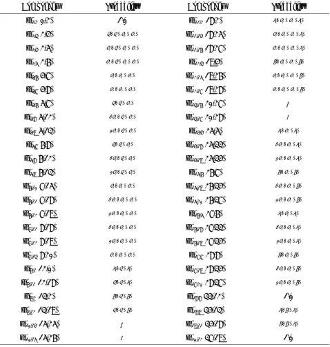
TABLE 5. Non-zero Components of Matrix U'. Probability Component Probability Component 1 2 /( )
ν μ +μ ν+
u′11,2(18,2)
1.0 u′1,2(0,2)
1/( 1 2 )
μ μ+μ ν+
u′11,14(18,25)
1 2
/( )
λ λ μ+ +μ
u′2,3(2,4)
2/( 1 2 )
μ μ +μ ν+
u′11,16(18,27)
1/( 1 2)
μ λ μ+ +μ
u′2,4(2,5)
1 2
/( )
θ μ+μ +θ
u′12,3(19,4)
2/( 1 2)
μ λ μ+ +μ
u′2,5(2,6)
1/( 1 2 )
μ μ +μ +θ
u′12,15(19,26)
1/( 1 2)
μ μ+μ
u′3,6(4,7)
2/( 1 2 )
μ μ +μ +θ
u′12,17(19,28)
2/( 2 2)
μ μ +μ
u′3,7(4,8)
a u′13,16(20,27)
2
/( )
λ λ μ+
u′4,6(5,7)
b u′13,17(20,28)
2/( 2)
αμ λ μ+
u′4,8(5,12)
2
/( )
ν μ ν+
u′14,4(25,5)
2/( 2)
βμ λ μ+
u′4,9(5,13)
2/( 2 )
αμ μ ν+
u′14,18(25,33)
1
/( )
λ λ μ+
u′5,7(6,8)
2/( 2 )
βμ μ ν+
u′14,19(25,34)
1/( 1)
αμ λ μ+
u′5,8(6,12)
2
/( )
θ μ +θ
u′15,6(26,7)
1/( 1)
βμ λ μ+
u′5,9(6,13)
2/( 2 )
αμ μ +θ
u′15,19(26,34)
1/( 1 2)
μ μ+μ
u′6,10(7,15)
2/( 2 )
βμ μ +θ
u′15,20(26,37)
2/( 1 2)
αμ μ+μ
u′6,11(7,18)
1
/( )
ν μ ν+
u′16,5(27,6)
2/( 1 2)
βμ μ +μ
u′6,12(7,19)
1/( 1 )
αμ μ ν+
u′16,18(27,33)
1/( 1 2)
αμ μ +μ
u′7,11(8,18)
1/( 1 )
βμ μ ν+
u′16,19(27,34)
1/( 1 2)
βμ μ+μ
u′7,12(8,19)
1
/( )
θ μ θ+
u′17,7(28,8)
2/( 1 2)
μ μ +μ
u′7,13(8,20)
1/( 1 )
αμ μ θ+
u′17,19(28,34)
/( )
ν λ ν+
u′8,1(12,0)
1/( 1 )
βμ μ θ+
u′17,20(28,37)
/( )
λ λ ν+
u′8,11(12,18)
1.0 u′18,8(33,12)
/( )
θ λ θ+
u′9,2(13,2)
/( )
ν θ ν+
u′19,9(34,13)
/( )
λ λ θ+
u′9,12(13,19)
/( )
θ θ ν+
u′19,11(34,18)
a
u′10,14(15,25)
1.0 u′20,12(37,19)
b
u′10,15(15,26)
simple structure of the model, all four blocks are quite sparse (few of the entries are non-zero). Table 4 reports the non-zero values of all these
matrices, with the understanding that xi,j(r,s)
to the transition probability from state r to state s. Using the method outlined by Equation 5, the transition probability matrix of the REMC reported in Table 5 is obtained. Solving the system of linearEquation 4, the steady state probabilities are obtained for all the states of the REMC. Supposing that the transition weights assume the following values: λ = 0.2, μ1 = 2.0, μ2 = 1.0, θ = 0.1, ν = 5.0, α
= 0.99, and β = 0.01. Using Equations 19 and 20, it is obtained: Security = 0.7078 and Reliability = 0.678.
8. CONCLUSION AND FUTURE WORKS
In this paper, we presented a method to derive non-functional parameters from the Generalized Stochastic Petri Net. These parameters can be a good guidance for selecting sufficient software models between recommended software models, to achieve a model with a high security, reliability. We use GSPN because it’s a formal model and there are many methods for transforming UML (which is widely used for modeling the system). There are some key activities to achieve this goal: Driving the CTMC from GSPN; which is extensively described in this paper by analyzing the CTMC then by obtaining the non-functional parameters. The work can be improved by integrating these steps in a CASE tool. It can also be expanded by mapping other UML diagrams to GSPN models.
9. REFERENCES
1. Robert, G,. Pettit, IV. and Gomaa, H., “Validation of Dynamic Behavior in UML Using Colored Petri Nets”, UML, Dynamic Behavior Workshop, York, England, (October, 2000).
2. Merseguer, J., L´opezGrao, J. P. and Campos, J., “From UML Activity Diagrams to Stochastic Petri Nets: Application to Software Performance Engineering”,
ACM, WOSP 04, California, (January, 2004).
3. Ajmone Marsan, M., “Modeling with Generalized Stochastic Petri Nets”, John Wiley Series in Parallel Computing-Chichester, (1995).
4. Motameni, H., Movaghar, A. and Mozafari, M., “Evaluating UML State Diagrams Using Colored Petri Net”, Proc. of SYNASC'05, Romania, (2005).
5. Trowittzsch Zimmermann, A. and Hommel, G., “Toward Quantitative Analysis of Real-Time UML
using Stochastic Petri Nets”, IPDPS, Colaorado, (2005).
6. S. Bernardi, S. Donatelli and J. Merseguer, “From UML Sequence Diagrams and State Charts to Analysable Petri Net Models”, ACM Proc. Int’l Workshop Software and Performance, (2002), 35-45.
7. Merseguer, J., Campos, J. and Mena, E., “Performance Analysis of Internet Based Software Retrieval Systems using Petri Nets”, ACM, Colaorado, (2001).
8. King, P. and Pooley, R., “Using UML to derive Stochastic Petri Net Models”, UKPEW, Bristol, (1999). 9. Merseguer, J., Bernardi, S., Campos, J. and Donatelli,
S., “A Compositional Semantics for UML State Machines Aimed at Performance Evaluation”, M. Silva, A. Giua and J. M. Colom (Eds.), Proc. of the 6th Int. Workshop on Discrete Event Systems (WODES'02),
Zaragoza, Spain, (2002), 295-302.
10. Elkoutbi, M. and Keller, R. K., “Modeling Interactive Systems with Hierarchical Colored Petri Nets”,
Advanced Simulation Technologies Conf., Boston,
MA, (1998), 432- 437.
11. Eshuis, R., “Semantics and Verification of UML Activity Diagrams for Workflow Modeling”, Ph.D. Thesis, University of Twente, (2002).
12. Fukuzawa, K. and Saeki, “Evaluating Software Architecture by Colored Petri Net”, Dept. of Computer Science, Tokyo Institute of Technology, Okayama 2-12-1, Meguro-uk, Tokyo, 152-8552, SDkE, Japan, (2002).
13. Pettit, R. G. and Gomaa, H., “Validation of Dynamic Behavior in UML Using Colored Petri Nets”, UML,
York, England, (2000).
14. Shin, M. E., Levis, A. H. and Wagenhals, L. W., “Transformation of UML-Based System Model into CPN Model for Validating System Behavior”, Proc. Compositional Verification of UML Models, Workshop, Sixth International Conference on the UML, San Francisco, CA, (October, 2003), 397-404.
15. Faul, M. B., “Verifiable Modeling Techniques Using a Colored Petri Net Graphical Language”, Technology Review Journal, Spring/Summer, (2004).
16. Motameni, H., Movaghar, A. and Kardel, B., “Verifying and Evaluating UML Activity Diagram by Converting to CPN”, Proc. of SYNASC'05, Romania, (2005).
17. Motameni, H., Zandakbari, M. and Movaghar, A., “Deriving Performance Parameters from the Activity Diagram Using GSPN and Markov Chains”, ICCSA 2006 Proceedings of 4th International Conference on Computer Science and Its Applications, San Ddiego,
California, USA, (2006).
18. Motameni, H., Montazeri, H., Siasifar, M., Movaghar, A. and Zandakbari, M., “Mapping State Diagram To Petri Net : An Approach To Use Markov Theory For Analyzing Non-Functional Parameters”, CISSE’06 Proceedings of 2th IEEE International Conferences on Computer, Information, and Systems Sciences, and Engineering, Bridgeport, USA, (2006).
20. Rana, O. F. and Shields, M. S., “Performance Analysis of Java Using Petri Nets”, Proceedings of the 8th International Conference on High-Perfromance Computing and Networking, (May, 2000), 657-667.
21. Choi, J. Y. and Reveliotis, S. A., “A Generalized Stochastic Petri Net Model for Performance Analysis and Control of Capacitated Re-entrant Lines”, IEEE Transactions on R and A, Vol. XX, No. Y, (2003).
22. Object Management Group, UMLTM Profile for Schedulability, Performance, and Time Specification, OMG document, Version 1.1, (January, 2005).