PRESENTING A MODIFIED SPH ALGORITHM FOR
NUMERICAL STUDIES OF FLUID-STRUCTURE
INTERACTION PROBLEMS
S. M. Hosseini and N. Amanifard*
Department of Mechanical Engineering, Faculty of Engineering University of Guilan, P.O.Box 3756, Rasht, Iran
*Corresponding Author
(Received: April 2, 2007 – Accepted in Revised Form: May 31, 2007)
Abstract A modified Smoothed Particle Hydrodynamics (SPH) method is proposed for fluid-structure interaction (FSI) problems especially, in cases which FSI is combined with solid-rigid contacts. In current work, the modification of the utilized SPH concerns on removing the artificial viscosities and the artificial stresses (which such terms are commonly used to eliminate the effects of tensile and numerical instabilities) as well as decreasing the CPU time with achieving more accuracy and the easier programming in comparison with other methods in the similar cases. The mentioned performance of the proposed algorithm is assessed by solving a test case including deformation of an elastic plate subjected to time-dependent water pressure. The obtained results are in close agreement with other high accuracy methods and experimental results.
Keywords Smoothed Particles Hydrodynamics (SPH), Fluid-Structure Interaction (FSI) Models, Lagrangian Method, Solid-Rigid Contact, Deformation of an Elastic Plate
ﻩﺪﻴﻜﭼ
ﺵﻭﺭﻩﺩﺍﻮـﻧﺎـﺧﺯﺍﻩﺪـﺷﺡﻼﺻﺍﻢﺘﻳﺭﻮﮕﻟﺍﮏﻳ
"
ﻞﺼـﺘﻣﺕﺍﺭﺫﮏﻴﻣﺎﻨﻳﺩﻭﺭﺪـﻴﻫ
" (SPH) ﻞﺋﺎﺴـﻣﯼﺍﺮـﺑ
ﺖﺳﺍﻩﺪﻳﺩﺮﮔﯽﻓﺮﻌﻣﻑﺎﻄﻌﻧﺍﻞﺑﺎﻗﻩﺭﺍﻮﻳﺩﻭﻝﺎﻴﺳﺶﻨﮐﺭﺪﻧﺍ
. ﯼﺯﺎﺠﻣﯽﺟﺰﻟﻑﺬﺣﺮﺑﺵﻭﺭﺡﻼﺻﺍ،ﻁﺎﺒﺗﺭﺍﻦﻳﺍﺭﺩ
ﺖﺳﺍﻩﺪﻳﺩﺮﮔﺭﺍﻮﺘﺳﺍﯼﺯﺎﺠﻣﯼﺎﻫﺶﻨﺗﻭ
:
ﺎﻫﺵﻭﺭﻩﺩﺍﻮﻧﺎﺧﺭﺩﻥﻮﻨﮐﺎﺗﻪﮐﯽﺗﻼﻤﺟ
ﯼ
(SPH) ﻩﺭﺍﻮﻤﻫ ﯼﺍﺮﺑ
ﺶﻫﺎﮐ
ﺖﺳﺍﻩﺪﺷﻪﺘﻓﺮﮔﺭﺎﮐﻪﺑﯼﺩﺪﻋﯼﺎﻫﯼﺭﺍﺪﻳﺎﭘﺎﻧ
.
ﺵﻭﺭﯼﺮـﻴﮔﺭﺎـﮐﻪـﺑﺭﺩﺮﺘﺸـﻴﺑﺖﻟﻮﻬـﺳﺮـﻣﺍﻦﻳﺍﺪﻣﺎﻴﭘ
(SPH)
ﻭ
ﺎﺘﺠﻴﺘﻧ
"
ﺖﺳﺍﯼﺩﺪﻋﻞﺣﯼﺍﺮﺟﺍﻥﺎﻣﺯﺶﻫﺎﮐﻭﯽﺴﻳﻮﻧﻢﺘﻳﺭﻮﮕﻟﺍ
. ﻞﺋﺎﺴـﻣﺯﺍﻪـﻧﻮﻤﻧﻪﻠﺌﺴﻣﮏﻳﯼﺍﺮﺑﻩﺪﺷﺩﺎﻳﺵﻭﺭ
ﺖﻴﻠﺑﺎﻗﻥﺩﺍﺩﻥﺎﺸﻧﯼﺍﺮﺑﻩﺭﺍﻮﻳﺩﻭﻝﺎﻴﺳﺶﻨﮐﺭﺪﻧﺍ
ﻉﻮﻧﺮﻫﻥﻭﺪﺑﻩﺭﺍﻮﻳﺩﮏﻴﺘﺳﻻﺍﻩﻭﺪﺤﻣﻭﻥﺎﻳﺮﺟﻡﺍﻮﺗﻞﺣﺭﺩﻥﺁ
ﺪﺷﻪﺘﻓﺮﮔﺭﺎﮐﻪﺑﯽﻧﺎﻴﻣﯼﺯﺮﻣﻁﺮﺷﺯﺍﻩﺩﺎﻔﺘﺳﺍ ﻩ
ﻩﺪﺷﺡﻼﺻﺍﺮﻴﻏﺵﻭﺭﺎﺑﺞﻳﺎﺘﻧﻭ
(SPH) ﻪﺴـﻳﺎﻘﻣﯽﺑﺮﺠﺗﺞﻳﺎﺘﻧﻭ
ﺖﺳﺍﻩﺪﻳﺩﺮﮔ
.
ﺎﻘﺗﺭﺍﺯﺍﯽﮐﺎﺣﻪﺴﻳﺎﻘﻣ ﯼ
(SPH)
ﺖﺤﺻ ﺞﻳﺎﺘﻧ ﺖﺳﺍ
.
1. INTRODUCTION
One of the interesting problems in many engineering applications is associated with solid boundary deformations due to the fluid flow. Both problems of viscous fluid flow and of elastic body deformation have been studied separately for many years in great detail. But there are many problems encountered in real life where an interaction between those two media is of great importance. Many tubes used in industries can have deformations due to interactions with other devices or to the degradation of the material constituting the tubes. A typical example of such a problem is the area of aero-elasticity. Another important area
where such interaction is of great interest is biomechanics. Such interaction is encountered especially when dealing with the blood circulatory system. Problems of a pulsatile flow in an elastic tube, flow through heart valves, flow in the heart chambers are some of the examples. In all these cases large deformations of a deformable solid interacting with an unsteady, often periodic, fluid flow must be dealt with [1].
walls and heart muscles are compliant and therefore play an important role in the process of opening and closing. Altogether, the combination makes the problem extremely complex to model [2].
Different ways of modeling fluid-structure interaction (FSI) have been proposed in the past, each having its advantages and disadvantages. Arbitrary Lagrangian Eulerian (ALE) methods, as exploited by e.g. [3,4], are most commonly used for FSI problems and have the advantage to provide a strong coupling. As long as rotations, translations and/or deformations of the solid remain within certain limits, this method works well and is recommended. However, for problems in which these limits are violated, elements become ill-shaped and ALE alone does not suffice. As a solution to this problem an often-used combination is ALE with some form of remeshing. This can, however, be a difficult and time consuming task.
A more elegant way to solve the system allowing free movement of a structure through a fluid domain was proposed by Peskin [5]. He introduced a method that later became known as the immersed boundary method (IBM) where flow-induced solid body motions could be computed without adjusting the fluid grid/mesh.
A method that could cope with large translations and rotations was used by Glowinski et al. [6,7]. Using a fictitious domain method, the sedimentation of rigid particles in a fluid domain could be computed. The rigid particles are immersed on the fluid domain and are coupled to the fluid by applying constraints across the particle using a Lagrange multiplier. This way of coupling is allowed for large translations as well as rotations of particles.
A method that resembles the above mentioned methods was introduced by Baaijens [8] for slender deforming bodies. In this method a fluid mesh is considered with an immersed solid mesh, and the solid mesh and fluid mesh are coupled by a Lagrange multiplier (or local body forces) at the boundary of the solid. The elegance of this method is its simplicity and flexibility. Actual three-dimensional approximation is, up to now, very rare. The most common approach is the combination of separate solvers for fluid and solid by an outer coupling iteration.
Another class of the fluid structure interaction
modeling is the fluid–solid mixture model which at first was applied to swelling and diffusion in rubber materials [9] and the compression of cartilage [10].
Nevertheless, it should be pointed out that the majority of the numerical schemes developed until now belong to the class of the so-called Eulerian methods, i.e. finite element (FE), finite volumes (FV), finite difference (FD) schemes, which make use of a fixed underlying grid to discretise the set of partial differential equations of the fluid motion. Until the early 1990s only a few works focused on the design of meshless methods for an alternative description of the physical problem, based on a purely Lagrangian description. Namely, many of these were concentrating more on astrophysical and cosmological problems, for whose simulations the first fully Lagrangian (and completely meshless) numerical method was developed in the late 1970s. This corresponds to the famous works of Lucy [11], Monaghan and Gingold [12] who in 1977 simultaneously and independently developed smoothed particle hydrodynamics (SPH).
free artificial viscosity SPH algorithm for simulating elastic solids and the fluid-structure interaction problems. It will be shown that the new algorithm can be utilized more easily with more accurate results for the test problems.
A benchmark of fluid-structure interaction problems was solved and the results are compared to the experimental results and the results of FEM simulation. The benchmark problem is the deformation of an elastic plate subjected to time-dependent water pressure.
2. FUNDAMENTALS
The SPH method is based on the interpolation theory. The method allows any function to be expressed in terms of its values at a set of disordered points representing particle points using a kernel function. The kernel function refers to a weighing function and specifies the contribution of a typical field variable,
A(r)
at a certain position,r
in space. The kernel estimate ofA(r)
is defined as [21]:( )
( ) (
Wr r,h)
dr Spacer A r
h
A = ∫ ′ − ′ ′ (1)
Where the smoothing length h represents the effective width of the kernel and W is a weighting function with the following properties [22]:
(
)
∫ − ′ ′=
V
1 r d h , r r
W W
(
r r,h) (
r r)
0hlim→ − ′ =δ − ′
(2) If A
( )
r′ is known only at a discrete set of N pointN r ,..., 2 r , 1
r then A
( )
r′ can be approximated as follows [28]:( )
r Nj 1 r rj A rj( )
dV jA ⎟
⎠ ⎞ ⎜ ⎝ ⎛
∑ = ⎟
⎠ ⎞ ⎜ ⎝ ⎛ −′ δ =
′ (3)
Where
( )
dV j is the differential volume element around the point rj. Combining Equation 1 and Equation 3 yields [28]:( )
r Nj 1 r rj A rj( ) (
dV jW r r,h)
dr hA ∑ = ∫ ⎟ − ′ ′
⎠ ⎞ ⎜ ⎝ ⎛ ⎟ ⎠ ⎞ ⎜ ⎝ ⎛ −′ δ =
(4) After integration, and replacing the differential
volume element
( )
dV j by mj ρj one gets [28]:( )
Nj 1 AjW(
r r,h)
j j m r
h
A =∑ = ρ − ′ (5)
Where the summation index j denotes a particle label and particle j carries a mass mj at position rj, a density ρj and a velocity vj. The value of A at j-th particle is shown by Aj. The summation is over particles which lie within a circle of radius 2h centered at r.
2.1. Kernel Function
The kernel function is themost important ingredient of the SPH method. Various forms of kernels with different compact support were proposed by many researchers. Recent studies [13,15,16] indicate that stability of SPH algorithm depends strongly upon the second derivative of the kernel.
Using different kernels in the SPH method is similar to using different schemes in finite difference methods. One of the most popular kernels is based on spline functions [17]:
( )
h r s s
2 0
2 s 1 3
) s 2 ( 4 1
1 s 0 3 s 4 3 2 s 2 3 1
h h ,r
W =
⎪ ⎪ ⎪
⎩ ⎪⎪ ⎪
⎨ ⎧
≤ < ≤ −
< ≤ +
−
× ν σ =
(6) Where ν is the number of dimensions and σ is
normalization constant with the values:
π π
1 , 7 10 , 3 2
2.2. Gradient and Divergence
The gradientand divergence operators need to be formulated in a SPH algorithm if simulation of the Navier-Stokes equations is to be attempted. In this work, the following commonly used forms are employed for a gradient of a scalar A and divergence of a vector u [22]:
ij W i
j j2
j A 2 i i A j m A i i 1 ∇ ∑ ⎟ ⎟ ⎟ ⎠ ⎞ ⎜ ⎜ ⎜ ⎝ ⎛ ρ + ρ = ∇
ρ (7)
ij W i
j j2
j u 2 i i u j m i u . i i 1 ∇ ∑ ⎟ ⎟ ⎟ ⎠ ⎞ ⎜ ⎜ ⎜ ⎝ ⎛ ρ + ρ = ∇
ρ (8)
Where ∇iWij is the gradient of kernel function
⎟ ⎠ ⎞ ⎜
⎝
⎛ −ir rj,h
W with respect to ri, the position of particle i. This choice of discretization operators ensures that an exact projection algorithm is produced.
2.3. Laplacian Formulation
A simple way toformulate the Laplacian operator is to envisage it as a dot product of the divergence and gradient operators. This approach proved to be problematic as the resulting second derivative of the kernel which is very sensitive to particle disorder and can easily lead to pressure instability and decoupling in the computation due to the co-location of the velocity and pressure. In this paper, the following alternative approach is adopted [23]:
∑ η + ∇ ⎟ ⎠ ⎞ ⎜ ⎝
⎛ρ +ρ
= ⎟⎟ ⎠ ⎞ ⎜⎜ ⎝ ⎛ ∇ ρ ∇
j 2 2
ij r ij W i . ij r ij A 2 j i 8 j m i A 1
. (9)
Where Aij=Ai−Aj,rij= ir−rj and η is a small number introduced to avoid a zero denominator during computations and is set to 0.1h.
3. GOVERNING EQUATIONS
In this paper a new algorithm for elastic
deformation modeling of solid particles is presented which doesn't utilize any artificial viscosity and artificial stress terms. The proposed algorithm for solid particle modeling is completely compatible with fluid particles and it Permits to easily follow the motion of fluid-solid interface in time without any specific treatment.?????
3.1. Governing Differential Equations for
Fluid Particles
The governing equations fortransient compressible fluid flow include the conservation of mass and momentum equations. In a Lagrangian framework these can be written as [27]:
0 v . Dt D
1 ρ+∇ =
ρ (10)
P 1 . 1 g Dt v D ∇ ρ − ⇒ τ ∇ ρ +
= (11)
Where t is time, g is the gravitational acceleration, P is pressure, v is the velocity vector, ⇒τ is viscous stress tensor and D/Dt refers to the material derivative. The density ρ has been intentionally kept in the equations to be able to enforce the incompressibility of the fluid. The momentum equations include three driving force terms, i.e., body force, forces due to divergence of stress tensor and the pressure gradient. These must be handled along with the incompressibility constraint. In a SPH formulation the above system of governing equations must be solved for each particle at each time-step. The sequence with which the force terms are incorporated can be different from one algorithm to another.
3.2. Viscous Terms in Fluid Zone
It isknown that In the Newtonian fluids, ⇒τ in Equation 11 must be defined as below:
D 2μ = ⇒
τ (12)
⎟ ⎠ ⎞ ⎜ ⎝ ⎛∇ +∇
= 12 v vt
D (13)
j v i u
⇒
τ in the momentum equation appears as a divergence form which can be written in SPH formulation as below [28]:
⎟ ⎠ ⎞ ⎜ ⎝ ⎛ − ∇ ⎟ ⎟ ⎟ ⎟ ⎠ ⎞ ⎜ ⎜ ⎜ ⎜ ⎝ ⎛ ρ ⇒ τ + ρ ⇒ τ ∑ = ⎟ ⎟ ⎠ ⎞ ⎜ ⎜ ⎝ ⎛ ⇒ τ ∇
ρ 2 . W ir rj,h j j 2 i i j j m i .
1 r r (15)
3.3. Governing Differential Equations for
Elastic Solid Zone
The acceleration equations(Momentum equation) for Elastic Medium can be written as below [19]:
⇒ σ ∇ ρ + = g 1 . t
d v d
(16)
In the above equations d/dt denotes a derivative following the motion, σ is the stress tensor and can be written as [19]:
ij S ij P ij=− δ +
σ (17)
By Combining Equation 16 and Equation 17 the final form of governing equations for Elastic Medium Motion includes the continuity and the acceleration equations which can be written as below 0 v . Dt D
1 ρ+∇ =
ρ (18)
P 1 S . 1 g t d v d ∇ ρ − ⇒ ∇ ρ +
= (19)
Where g is the gravitational acceleration, P is pressure, ⇒S is the deviatoric stress tensor and its rate of change is given by [19]:
kj S ik jk ik S ij ij 3 1 ij 2 t d ij S
d + ω +ω
⎟ ⎠ ⎞ ⎜
⎝
⎛ε − δ ε μ
= & & (20)
Where [19]: ⎟ ⎟ ⎠ ⎞ ⎜ ⎜ ⎝ ⎛ ∂ ∂ + ∂ ∂ = ε i x j v j x i v 2 1 ij
& (21)
and the rotation tensor ωij is [19]:
⎟ ⎟ ⎠ ⎞ ⎜ ⎜ ⎝ ⎛ ∂ ∂ − ∂ ∂ = ω i x j v j x i v 2 1
ij (22)
4. SOLUTION ALGORITHM
In this paper, a fully explicit three-step algorithm is used for both fluid and elastic solid particles which will be explained in detail.
4.1. Solution Algorithm for Fluid
Particles
In the first step of this algorithm, themomentum equation is solved in the presence of the body forces neglecting all other forces. So, an intermediate velocity is computed as
t x g t t u *
u = −Δ + Δ (23)
t y g t t v *
v = −Δ + Δ (24)
As said before, in the second step of fluid flow simulation the temporal velocity is employed to calculate the divergence of viscous stress tensor. Note that the divergence of viscous stress tensor is a vector Tr given by:
j y T i x T T i .
1 =r = r + r
⎟ ⎟ ⎠ ⎞ ⎜ ⎜ ⎝ ⎛ ⇒ τ ∇
ρ (25)
At the end of the second step, the particle velocity is updated according to
t x T t x g t t u t x T * u * *
u = + Δ = −Δ + Δ + Δ (26)
t y T t y g t v t y T * v * *
v = + Δ = + Δ + Δ (27)
At this stage the particle moved according to temporal velocities (u** ,v**) and temporal position of the particle is:
t * * u t t x *
t * * v t t y *
y = −Δ + Δ (29)
Thus far no constraint has been imposed to satisfy the incompressibility of the fluid and it is expected that the density of some particles change during this updating. In fact, with the help of the continuity equation one can calculate the density variations of each particle as
⎟ ⎠ ⎞ ⎜ ⎝ ⎛ ∇ ⎟ ⎠ ⎞ ⎜ ⎝ ⎛ − ∑ = ρ h , ij r W i . j v i v j j m Dt i D (30)
Where ρi and vi are the density and velocity of particle i. When two particles approach each other, their relative velocity and therefore the gradient of kernel function become negative, so Dρi Dt will be positive and ρi will increase. Consequently, this will produce a repulsive force between the approaching particles. In a similar fashion, if two particles are repulsed from each other, an attractive force will be produced to stop this. This interaction based on the relative velocity of particles and the resulting coupling between the pressure and density will enforce incompressibility in the solution procedure.
The velocity field vˆ=
( )
uˆ,vˆ which is needed to restore the density of particles to their original value is now calculated. To do this, in the third step of the algorithm, the momentum equation with the pressure gradient term as a source term is combined with the continuity Equation 10 as0 ) vˆ .( t * 0 0
1 +∇ =
Δ ρ − ρ
ρ (31)
t P * 1 vˆ Δ ⎟ ⎟ ⎠ ⎞ ⎜ ⎜ ⎝ ⎛ ∇ ρ −
= (32)
to obtain the following pressure of the Poisson equation 2 t 0 * 0 P * 1 . Δ ρ ρ − ρ = ⎟ ⎟ ⎠ ⎞ ⎜ ⎜ ⎝ ⎛ ∇ ρ
∇ (33)
Equation 35 can be discretized according to Equation 9 to obtain pressure of each particle as
⎟⎟ ⎟ ⎟ ⎟ ⎟ ⎠ ⎞ ⎜⎜ ⎜ ⎜ ⎜ ⎜ ⎝ ⎛ ⎟⎟ ⎟ ⎟ ⎟ ⎟ ⎠ ⎞ ⎜⎜ ⎜ ⎜ ⎜ ⎜ ⎝ ⎛
η
+
∇
∑
ρ
+
ρ
η
+
∇
∑
ρ
+
ρ
+
Δ
ρ
ρ
−
ρ
=
2
2
j
i
r
ij
W
i
.j
i
r
j
(
i
j
)
2
j
m
8
2
2
j
i
r
j
i
W
i
.j
i
r
j
P
j
(
i
j
)
2
j
m
8
2
t
0
*
0
i
P
r
r
r
r
(34) using this value for the pressure of each particle onecan calculatevˆ according to Equation 34 and 7 as
ij W i ) 2 j j P * 2 i i P ( j j m i vˆ ∇ ρ + ρ ∑
= (35)
Finally, overall velocity of each particle at the end of the time step will be obtained as
uˆ * * u t t
u +Δ = + (36)
vˆ * * v t t
v +Δ = + (37)
And the final positions of particles are calculated using a central difference scheme in time
) t t u t u ( 2 t t t x t
x = −Δ +Δ + −Δ (38)
) t t v t v ( 2 t t t y t
y = −Δ +Δ + −Δ (39)
4.2. Solution Algorithm for Solid
Particles
A comparison between governingequations of fluid and solid zones shows that only the second term in momentum equations differ from each other. So, just the second step of solution algorithm for solid particles is different from related step in fluid particles.
calculating ε&ij and ωij (Equations 21 and 22). To model an elastic-plastic material an additional yield condition is required which defines the material elastic limit and hence determines when plastic flow occurs. For the present work, the von Mises yield condition has been employed, which can be written in terms of the principal stresses, By using the yield strength of the material in simple tension (τY), the yield condition can be written as [25]
2 Y 2 xy S 2 2 y S 2 x
S + + ≤τ (40)
and it is this expression which is used here to detect the onset of plastic flow. In the numerical scheme discussed in this work, once yield is detected the material is assumed to flow plastically, resisting with a constant state of deviatoric stress; hence the term elastic-perfectly plastic.
If the above condition is satisfied then response is elastic and this is the final state of stress, otherwise the material has yielded and flow is plastic and each stress component must be rescaled to lie on the yield surface by multiplying by the rescaling factor [24]:
2 xy S 2 2 y S 2 x S
Y 3 2
+ +
τ
(41)
Similar to the second step for the fluid zone, the divergence of deviatoric stress is utilized for calculating the temporal velocities (u** ,v**), then temporal position (x*,y*) of particles will be calculated at the end of the second step. The third step for satisfying the incompressibility to elastic solid particles is completely similar to fluid ones. It should be mentioned that all of the SPH algorithm for simulating solid particles utilizes an artificial viscosity term (in order to smooth out the velocity oscillations) and artificial stress (to eliminate the effects of tensile instability) but none were used in the artificial parameters in this new algorithm. In addition the pressures of solid particles are calculated by solving continuity with the third term of momentum equation (in third step of proposed algorithm) instead of using the equation.
5. FLUID-STRUCTURE INTERACTION MODEL
In the first attempt of the fluid-structure interaction modeling with SPH [20], some particles were defined as interface particles. The way to define the interface and its normal vector was similar to that which was proposed by [25] to define complex solid boundaries. The dynamic interface conditions were satisfied by adding some source terms to the momentum equation which is equivalent to the action-reaction principle. It was guaranteed that by imposing the force exerted by the fluid on the solid the same modulus as the force exerted by the solid, an opposite force is exerted to the fluid.
Here a different method for Fluid-structure interaction modeling is proposed. In this method it was assume that in each time step, elastic walls play the role of rigid walls for fluid particles and only contribute in the third step of computational algorithm. In fact, when fluid particles move toward elastic particles their pressure increases and prevents them from penetrating into a solid zone. Because of using the same solution algorithm for both fluid and solid zones, it can be assumed that a similar effect on solid particles due to fluid flow would take place. In another words, fluid particles contribute only in the third step of the solution procedure of their solid neighbors.
It will be shown that the accuracy of presented the method is higher than the old one. It has other advantages such as: easier implementation, no special treatment for interface particles, less CPU time (it hasn’t any extra procedure for interface calculation).
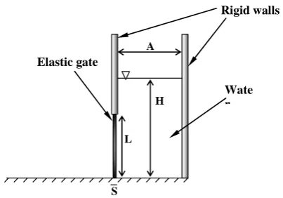
6. RIGID WALL BOUNDARY CONDITIONS
Rigid walls
Elastic gate
Wate r
A
L H
S
Figure 1. Schematic view of initial configuration. completely similar to boundary particles are also
placed outside of the solid walls at spacing l0. The calculation procedure for both wall and dummy particles is completely similar to inner particles, except the zero velocity for no slip boundary conditions.
7. THE TEST CASE
In this section, a benchmark problem is studied to demonstrate the capability of the proposed method to solve fluid-structure interaction problems. The benchmark problem is the deformation of an elastic plate subjected to time-dependent water pressure.
The results are compared with experimental data and results of the first attempt of SPH-FSI model [20] to show the better accuracy of the proposed algorithm.
Throughout this study and whatever the chosen smoothing length value, the typical distance (notedΔx) between two particles is determined so
that the interpolation circle contains about 20 particles (in a two dimensional context), that is,
15 . 1 x h =
Δ (42)
It should be mentioned that the formulation utilized for elastic wall simulation is comparable with a fluid with large viscosity (with the order of G), so the particles in the elastic solid zone have to be arranged closer to each other in comparison to fluid particles. In this simulation the initial spacing between solid particles is half of fluid ones, it means, the number of particles for showing the same amount of mass for an elastic solid zone is 2 times greater than a fluid one.
An elastic gate, clamped at one end and free at the other one, interacts with a mass of water initially confined in a free-surface tank behind the gate. A schematic view of this 2D problem is shown in Figure 1. As it is shown, the left wall consists in an upper rigid part and in a lower deformable plate made of rubber. The rubber plate is free at its lower end, thus representing an elastic gate closing the tank. The geometric dimensions of the system and the physical characteristics of the
elastic gate are reported in Table 1.
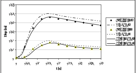
In Figure 2, the horizontal and vertical displacements computed for the plate (according to the presented SPH algorithm and FSI model) are compared with those measured in the digitalized images acquired during the experiments and the results of old SPH model of FSI.
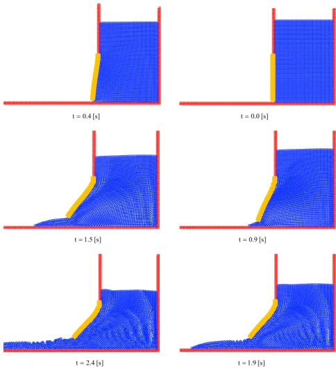
Water level just behind the gate is shown in Figure 3. SPH particle positions at six different times are shown in Figure 4. These images are in complete agreement with the frames from the experiment setup at corresponding times (shown in [20]).
The evolution of the free-surface is also well reproduced by the simulation. Figure 4 shows the water level history immediately behind the gate. As it can be seen, the accuracy of presented SPH simulation is completely greater than the old one. It is because of using a better algorithm for solid elastic simulation and no special treatment for interface particles (the interface modeled naturally).
8. CONCLUSION
This paper presents a numerical investigation of a fluid-structure interaction (FSI) model according to a modified Smoothed Particle Hydrodynamics (SPH) method.
TABLE 1. Dimensions of the System and Physical Characteristics of the Rubber Plate. Dimensions
A (m) 0.1
H (m) 0.14
L (m) 0.079
S (m) 0.005
Rubber
ρ (kg/m3) 1100
G (N/m2) 4.27 × 10 6
0 0.01 0.02 0.03 0.04 0.05 0.06
0 0.05 0.1 0.15 0.2 0.25 0.3 0.35 0.4 t [s]
Di
sp
[
m
]
Experiment -x Old-SPH-x Experiment-y Old-SPH-y Present-SPH-x Present-SPH-y
Figure 2. Horizontal and vertical displacements of the free end of the plate.
0 0.02 0.04 0.06 0.08 0.1 0.12 0.14 0.16
0 0.1 0.2 0.3 0.4 t [s]
y [
m
] Experiment
Old-SPH Present-SPH
Figure 3. Water level (m) just behind the gate. frame. The modification of the utilized SPH
concerns on removing the artificial viscosities and the artificial stresses (which such terms are commonly used to eliminate the effects of tensile and numerical instabilities). The new algorithm for elastic simulation is based on a prediction-correction procedure which has been used for fluid flow simulation. According to the presented method pressure Poisson equation (Equation 35) is utilized for pressure calculation instead of state equation which has some dependent constant to the materials and dynamics of the problems.
However, the purpose of this work was to propose a different method for Fluid-structure interaction modeling in engineering applications. It was shown that this method has some advantages
such as more accuracy and easier programming compared to other methods in similar cases. The mentioned performance of the proposed algorithm is assessed by solving a test case including deformation of an elastic plate subjected to time-dependent water pressure. The obtained results are in close agreement with other high accuracy methods and experimental results.
9. NOMENCLATURE
A A Typical Field Variable
]
s [ 4 . 0
t= t =0.0[s]
]
s [ 5 . 1
t = t=0.9[s]
]
s [ 4 . 2
t = t =1.9[s]
Figure 4. SPH particle positions at six different times.
W Weight Function (Kernel)
h Smoothing Length
V Volume
δ Dirac Delta Function
m Mass of Particle ρ Density v Velocity
s Normalized Position Variable
u Velocity Vector
V Velocity Vector
τ Viscous Stress Tensor g Gravity Force Per Unit Mass S Shear Strain
P Pressure
t Time
Δx Space Step
Subscripts
i Target Particle Index
j Neighborhood Particle Index
Y Yeilding Point
x Normal in x-Direction y Normal in y-Direction xy Shear Direction in x-y Plain.
0 Reference Values
t Time Index
Δt Time Step
Superscripts
*,** Temporal Variables
^ Field Variables
. Time Derivity
10. REFERENCES
1. Jaroslav Hron, Martin Mádlík, Fluid-structure interaction with applications in biomechanics, Nonlinear Analysis: Real World Applications”, Article In Press, (2006), 1431-1458.
2. Van Loon, R., Anderson, P. D. and Van De Vosse, F. N. “A fluid-structure interaction method with solid-rigid contact for heart valve dynamics”, Journal of Computational Physics, Vol. 217, (2006), 806-823. 3. Hirt, C. W., Amsden, A. A. and Cook, J. L. “An
arbitrary Lagrangian-Eulerian computing method for all speeds”, J. Comput. Phys., Vol. 14, (1974), 227-253. 4. Donea, J., Giuliani, S. and Halleux, J. P., “An arbitrary
Lagrangian-Eulerian finite element method for transient dynamic fluid-structure interactions”, Comput. Meth. Appl. Mech. Eng., Vol. 33, (1982), 689-723.
5. Peskin, C. S., “The immersed boundary method”, Act. Num., Vol. 11, (2002), 479-517.
6. Glowinski, R., Pan, T. W. and Pe´riaux, J., “A Lagrange
multiplier/fictitious domain method for the numerical simulation of incompressible viscous flow around moving rigid bodies”, C. R. Acad. Sci. Paris, Vol. 25, No. 5, (1997), 361-369.
7. Glowinski, R., Pan, T. W., Hesla, T. I. and Joseph, D. D., “A distributed Lagrange multiplier/fictitious domain method for particulate flows”, Int. J. Multiphase Flow, Vol. 324, (1999), 755-794.
8. Baaijens, F. P. T., “A fictitious domain/mortar element method for fluid–structure interaction”, Int. J. Num. Meth. Fluids,Vol. 35, No. 7, (2001), 743-761.
9. Dai, F. and Rajagopal, K. R. “Diffusion of fluids through transversely isotropic solids”, Acta Mech.,Vol. 82, (1990), 61-98.
10. Spilker, R. L., Suh, J. K. and Mow, V. C., “Finite element formulation of the nonlinear biphasic model for articular cartilage and hydrated soft tissues including strain-dependent permeability”, Comput. Meth. Bioeng, Vol. 9, (1988), 81-92.
11. Lucy, L. B., “A numerical approach to the testing of the fission hypothesis Astron”, J.of Astronomy, Vol. 82, 1013–24
12. Gingold, R. A. and Monaghan, J. J., “Smoothed particle hydrodynamics theory and application to non-spherical stars”, Mon. Not. R. Astronom. Soc., Vol. 181, (1977), 375.
13. Monaghan, J. J., “Simulating free surface flows with SPH”, J. Comp. Physics, Vol. 110, (1994), 399. 14. Chaniotis, A. K., Poulikakos, D. and Koumoutasakos,
P., “Remeshed smoothed particle hydrodynamics for the simulation of viscous and heat conducting flows”, J. Comp. Physics, Vol. 182, (2002), 67-90.
15. Owen, J. M., “Remeshed smoothed particle hydrodynamics for the simulation of viscous and heat conducting flows”, J. Comp. Physics, Vol. 182, (2002), 67-90.
16. Takeda, H., Miyama, S. M. and Sekiya, M., “Numerical Simulation of Viscous Flow by Smoothed Particle Hydrodynamics”, Progress of Theoretical Physics, Vol. 92, No. 5, (1994), 939-960.
17. Cleary, P., Ha, J., Alguine, V. and Nguyen, T., “Flow modelling in casting processes”, Applied Mathematical Modelling, Vol. 26, (2002), 171-190.
18. Oger, G., Doring, M., Alessandrini, B. and Ferrant, P., “Two-dimensional SPH simulations of wedge water entries”, J. Comp. Physics, (2005), 803-822.
19. Gray, J. P., Monaghan, J. J. and Swift, R. P.,“SPH elastic dynamics”, Comp. Methods Appl. Mech. Eng., Vol. 190, (2001), 6641-6662.
20. Antoci, C., Gallati, M. and Sibilla, S., “Numerical simulation of fluid-structure interaction by SPH”, Computers and Structures, (2007), 879-890.
21. Monaghan, J. J., “Smoothed particle hydrodynamics”, Annul. Rev. Astron. Astrophys., Vol. 30, (1992), 543-574.
22. Colagrossi, A. and Landrini, M., “Numerical simulation of interfacial flows by smoothed particle hydrodynamics”, J. Comp. Phys., Vol. 191, (2003), 448-475.
24. Howell, B. P. and Bally, G. J., “A Free-Lagrange Augmented Godunov Method for the Simulation of Elastic-Plastic Solids”, J. Comp. Phys., Vol. 175, (2002), 128-167.
25. Randles, P. W. and Libersky, L. D., “Smoothed particle hydrodynamics: some recent improvements and applications”, Comput Methods Appl Mech Eng, Vol. 139, (1996), 375-408.
26. Koshizuka, S., Oka, Y. and Tamako, H., “A particle method for calculating splashing of incompressible viscous fluid”, Internation Confe renc e on
Mathematics and Computations, Vol. 2, (1995), 1514-1526.
27. Edmond, S. S. and Lo, Y. M., “Incompressible SPH method for simulating Newtonian and non-Newtonian flows with a free surface”, Advances in Water Resources, Vol. 26, (2003), 787-800.