SEISMIC BEHAVIOR OF SILOS WITH DIFFERENT HEIGHT TO DIAMETER RATIOS CONSIDERING GRANULAR MATERIAL-STRUCTURE INTERACTION

(1)

SEISMIC BEHAVIOR OF SILOS WITH DIFFERENT HEIGHT TO

DIAMETER RATIOS CONSIDERING GRANULAR

MATERIAL-STRUCTURE INTERACTION

F. Nateghi and M. Yakhchalian*

Structural Engineering Research Center, International Institute of Earthquake Engineering and Seismology, Tehran, Iran

*Corresponding Author

(Received:َApril 09, 2011 – Accepted in Revised Form: December 15, 2011)

doi: 10.5829/idosi.ije.2012.25.01b.04

Abstract Silos are structures that are used for storing different types of granular material. Dynamic behavior of silos under seismic loads is very complex. In this paper seismic behavior of steel silos with different height to diameter ratios is investigated by considering granular material-structure interaction using ABAQUS finite element package. Silo wall is modeled by shell elements and its behavior is considered elastic, seismic behavior of granular material inside silo is highly nonlinear and requires a complex nonlinear description of the granular material. The hypoplasticity theory describes the stress rate as a function of stress, strain rate and void ratio. The granular material is modeled by solid elements and its behavior is considered with a hypoplastic constitutive model, for modeling of interaction between silo wall and granular material, surface to surface contact with coulomb friction law is considered between silo wall and granular material. The results show that the seismic behavior of silos is dependent on the height to diameter ratio of the silo. While considering a constant value for the distribution of acceleration in the height of silo leads to conservative design pressures for a squat silo based on Eurocode 8, this assumption is not conservative for a slender silo.

Keywords Steel silo; Seismic behavior; Finite element method; Hypoplasticity; Granular material-structure interaction; Surface to surface contact.

1. INTRODUCTION

Silos are structures which are used for storing granular materials like grain, coal and other granular materials. Silos should be designed against earthquake in earthquake-prone areas. During earthquake silo wall experiences additional

stresses resulting from unsymmetrical pressure distributions in the silo. In addition the dynamic loads lead to compaction of granular material inside silo. In silo design based on ACI 313 [1] wall pressures from such effects are not taken into account. The system is reduced to a cantilever beam with several point masses being situated on

راﺮﻗ هدﺎﻔﺘﺳا درﻮﻣ ياﻪﻧاد ﺢﻟﺎﺼﻣ ﻒﻠﺘﺨﻣ عاﻮﻧا ندﺮﮐ هﺮﯿﺧذ ياﺮﺑ ﻪﮐ ﺪﻨﺘﺴﻫ ﯽﯾﺎﻫهزﺎﺳ ﺎﻫﻮﻠﯿﺳ

هﺪﯿﮑﭼ

ياهزﺮﻟ رﺎﺘﻓر ﻪﻟﺎﻘﻣ ﻦﯾا رد .ﺖﺳا هﺪﯿﭽﯿﭘ رﺎﯿﺴﺑ ياهزﺮﻟ يﺎﻫرﺎﺑ ﺮﺛا ﺖﺤﺗ ﺎﻫﻮﻠﯿﺳ ﯽﮑﯿﻣﺎﻨﯾد رﺎﺘﻓر .ﺪﻧﺮﯿﮔﯽ ﻣ زا هدﺎﻔﺘﺳا ﺎﺑ هزﺎﺳ و ياﻪﻧاد ﺢﻟﺎﺼﻣ ﺶﻨﮐرﺪﻧا ﻦﺘﻓﺮﮔ ﺮﻈﻧرد ﺎﺑ ﻒﻠﺘﺨﻣ ﺮﻄﻗ ﻪﺑ عﺎﻔﺗرا يﺎﻬﺘﺒﺴﻧ ﺎﺑ يدﻻﻮﻓ يﺎﻫﻮﻠﯿﺳ دوﺪﺤﻣ ءاﺰﺟا راﺰﻓا مﺮﻧ ياﻪﺘﺳﻮﭘ يﺎﻬﻧﺎﻤﻟا زا هدﺎﻔﺘﺳا ﺎﺑ ﻮﻠﯿﺳ هراﻮﯾ د .ﺖﺳا ﻪﺘﻓﺮﮔ راﺮﻗ ﯽﺳرﺮﺑ درﻮﻣ ABAQUS

(2)

top of each other to calculate appropriate actual weight of stored material should be considered as effective weight for calculating 313 resulted from agreement among Committee 313 members who wrote the original standard but had not been verified by experiment at that time. Subsequently Harris and von Nad [2] performed shaking tests on relatively rigid steel model silos filled with sand and wheat. The effective weight 80 percent value considered in ACI 313. Eurocode 8 part 4 [3] considers additional horizontal pressures resulting from earthquake effects with simple relations. Eurocode 8 Part 4 has proposed that if more accurate evaluations are not undertaken, the global seismic response and the seismic action effects in the supporting structure may be calculated assuming that the particulate contents of the silo move together with the silo shell and modeling them with their effective mass, the contents of the silo may be taken to have an effective mass equal to 80 percent of their total mass.

There are few researches that have tried to investigate the behavior of silos under earthquake loading with considering granular material-structure interaction. Braun and Ebil [4] are the first researchers that have proposed hypoplasticity for modeling of granular material inside silos under earthquake loading. They have used a simple hypoplastic model. The behavior of granular material is incrementally nonlinear even at low strains. The hypoplasticity theory describes the stress rate as a function of stress, strain rate and void ratio. It can model the nonlinear and inelastic behavior of granular material. Holler and Meskouris [5] have tried to investigate the behavior of silos under earthquake loading. They have tested different hypoplastic models and concluded that von Wolffersdorf’s hypoplastic model [6] with intergranular strain extension [7] is the most effective material law for describing the time dependent cyclic behavior of granular material. The results of their research show that the provisions given in the Eurocode yield good results for the slender silos. While for squat silos the results are too conservative, the material parameters presented for granular material inside silo in their research lead to high values of stiffness for granular material inside silo. In this paper the

behavior of three steel silos with different height to diameter ratios considering granular material-structure interaction is investigated under earthquake excitation using von Wolffersdorf’s hypoplastic model with intergranular strain extension. Granular material inside silo models is considered to be a type of sand which parameters are available in technical literature.

2. PRESSURES UNDER EARTHQUAKE LOADING IN EUROCODE 8 PART 4

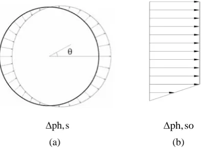
In Eurocode 8 part 4, it is mentioned that if the mechanical properties and the dynamic response of the particulate solid are not explicitly and earthquake effect should be represented through an additional normal pressure on the silo wall. In circular silos, the additional normal pressure on the wall may be taken as the following equation:

θ

Cos so ph, s

ph, =∆

∆ (1)

where

∆

ph,

so

is the reference pressure and θ is the angle between the radial line to the point of horizontal component of the seismic action. The distribution of

∆

ph,

s

in the section of silo is shown in Figure 1(a).

s ph,

∆ ∆ph,so

Figure 1. (a) The distribution of ∆ph,s in the section of silo, (b) The distribution of ∆ph,so in the height of silo

At points on the silo wall at a vertical distance

x

from a flat bottom or the apex of a conical or pyramidal hopper, the reference pressure ∆ph,so may be taken as:

(a) (b)

accurately counted for the analysis, the

interest on the wall and the direction of the additional static horizontal loads. About 80 percent of

masses. Also 80 percent effective weight in ACI

(3)

) 3 *, min( ) ( so

ph, =

α

z

γ

r_s x

∆ (2) )

(z

α

is the ratio of the response acceleration of the silo at a vertical distance z from the equivalent surface of the stored contents, to the acceleration of gravity.

γ

is the bulk unit weight of the particulate material in the seismic design situation.

*

s

r

is defined as below: ) 2 / , min(

* b c

s h d

r = (3)

b

h

is the overall height of the silo, from a flat bottom or the hopper outlet to the equivalent surface of the stored contents and

d

c is the inside dimension of the silo parallel to the horizontal component of the seismic action. The distribution of ∆ph,so in the height of silo by considering

) (z

α

equal to a constant value (The ratio of response acceleration at the center of gravity of the particulate material to the acceleration of gravity) is shown in Figure 1(b).

3. HYPOPLASTICITY THEORY FOR MODELING OF GRANULAR

MATERIAL

Hypoplasticity is a class of incrementally nonlinear constitutive models that are developed to predict the behavior of soils. The basic structure of the hypoplastic models has been developed during 1990's at the University of Karlsruhe. Hypoplasticity is a framework for the description of mechanical behavior of granular materials. The hypoplastic material laws describe the stress rate as a function of stress, strain rate and void ratio and are well for modeling of cohesionless granular materials. Hypoplasticity can model the nonlinear and inelastic behavior of soils due to its rate-type formulation that ensures a realistic modeling of loading and unloading paths. von Wolffersdorff’s hypoplastic constitutive model [6] can model the nonlinear behavior of granular materials very well but it has some drawbacks for application to cyclic loadings. The most significant shortcoming of this model is an excessive accumulation of deformations for small stress cycles that is called ratcheting. To solve this significant shortcoming, Niemunis and Herle [7] presented an extension for von Wolffersdorff’s hypoplastic constitutive model by introducing the intergranular strain concept. In

this paper von Wolffersdorff’s hypoplastic constitutive model with intergranular strain extension is used for modeling of granular material inside silo.

The general stress-strain relation in the hypoplastic model with intergranular strain concept is:

: =

T

M

D (4)

o

T is objective Jaumann stress rate, D is stretching rate and

M

is a fourth-order tensor that represents stiffness. The intergranular strain δ is obtained by accumulation of DΔt and is a second-order tensor.

ρ

is the normalized magnitude of δ.

R

δ

=

ρ (5)

is the Euclidean norm of a tensor (e.g.

ij ij

δ

= δ ). ^

δ is the direction of intergranular strain and is defined as below:







=

≠

=

0

δ

0

δ

^

for

/

(6)

Material stiffness can be calculated from the following equation:

[

]

    ≤ − > + − + − + = 0 : for : ) ( 0 : for : ) 1 ( ) 1 ( D δ δ δ D δ δ N δ δ ^ ^ ^ ^ ^ ^ ^ L L L M T R T R T m m m m m χ χ χ χ χ ρ ρ ρ ρ ρ (7)

The evolution equation for the intergranular strain tensor δ is:









≤

>

−

=

0

:

for

0

:

for

:

)

(

D

δ

D

δ

D

δ

_^ ^ ^ ^ r β

ρ

I

 (8)

L

is a fourth-order tensor and N is a second-order tensor. The constitutive tensors

L

and N are functions of stress and void ratio that are defined in Equations 9 and 10.

(4)

2 2

( )

: b e

1

= f f F + a

^ ^

^ ^ T T

T T

L I (9)

+ : d b e

Fa = f f f

^ ^

N (T T*)

T T

(10)

I

is the unit tensor of fourth-order.

tr

= /

^

T T T (11) T is the stress tensor.

1 3 =

-^ ^

T* T 1₍₁₂₎

1 is the unit tensor of second-order.

c c a φ φ sin 2 2 ) sin (3 3 −

= (13)

ψ θ ψ ψ ψ F tan 2 2 1 3 cos tan 2 2 tan 2 tan 8

1 2 2 −

+ − +

= (14)

tanψ = 3

^

T* (15)

3

2 3/ 2

tr( ) cos 3 6

[tr( )]

θ= −

^

^ T*

T*

(16)

In the above mentioned equations tensors of second-order are denoted with bold letters and tensors of fourth-order with calligraphic letters, in addition different kinds of tensorial multiplication are used (e.g.

M

:D=

M

_ijkl D_kl, ij kl

^ ^

δ

=

^ ^

δ

, kl ij

N

^

δ

=

^

δ

N

, ij

D

_ij

^

:

D

=

δ

^ ).

e

f

and

f

d are pycnotropy functions.

β       = e e f c

e (17) α       − − = d c d d e e e e

f (18)

b

f

is barotropy function.

1 0

0

1 2 0 0

0 0

1 tr

3 3

n

s i i

b

i c s

i d

c d

h e e

f

n e e h

e e a a e e β α − −  +   −  = _ _ _{ } _       _ ₋ _    × + − _ _ −  _ _    T (19)

These functions take into account the influence of density and mean pressure. Three characteristic void ratios

e

_i (during isotropic compression at the minimum density),

e

_c (critical void ratio) and

e

_d

(maximum density) decrease with mean pressure according to the following equation:

0 0 0

tr exp

n

i c d

i c d s

e e e

e e e h

 _₋ _    = = = _−   _ _    T (20)

von Wolffersdorff’s hypoplastic model requires eight material parameters.

φ

_c is critical friction angle, e_c₀ is the conventional maximum void ratio,

0

d

e is conventional minimum void ratio and e_i₀ is maximum possible void ratio at zero pressure. h_s is granular hardness that is a pressure-independent stiffness and n is an exponent, appearing in the power law for proportional compression.

α

and

β

are exponents to be calculated from the triaxial peak friction angle. Five additional material parameters are required for intergranular strain extension. R, m_R, m_T,

β

_r and

χ

are intergranular strain parameters. The parameter R is the maximum intergranular strain. The maximum value of intergranular strain can be found from stress-strain curves obtained either from so-called dynamic tests or from static tests with strain reversals. The incremental stiffness remains approximately constant within a certain strain range. The size of this range can be identified with the constant R. Factors m_R and m_T are the increase factors of stiffness for each load reversal in the 180 degrees and 90 degrees directions compared to the stiffness in the 0 degrees direction. In order to determine the constants m_R and m_T comparative tests at fixed values of T,

e

(5)

calibrated from cyclic test with small strain amplitudes. The parameter βr influences the

evolution of intergranular strain.

4. MODELING

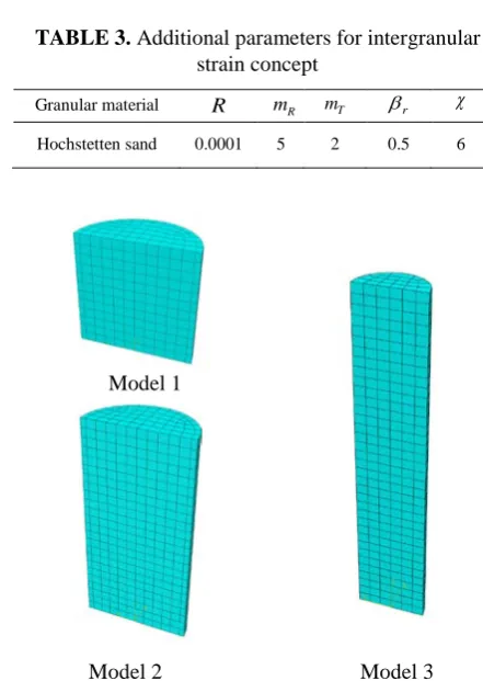
In this research three steel silos with different height to diameter ratios were considered. Hochstetten sand [8] was considered as granular material inside silos. The mass density of sand was considered equal to 1500 kg/m3. Dimensions of silo models are presented in Table 1. ABAQUS finite element package [9] was used for finite element modeling. von Wolffersdorff’s hypoplastic constitutive model with intergranular strain extension implemented in the form of UMAT [10] for ABAQUS was used for modeling of granular material inside silos. 8-noded solid element C3D8 was used for modeling of granular material inside silos. The parameters of hypoplastic model for sand are presented in Tables 2 and 3.

The initial value of void ratio considered for granular material inside silos was 0.7. 4-noded shell element S4 was used for modeling of silo wall and silo bottom. The Modulus of elasticity of steel wall of silos was considered equal to 2×105 MPa. For decreasing the computation time only half of silo was modeled and symmetric boundary conditions were used at the center of silo and granular material. The finite element mesh of silo models and granular material inside silos is shown in Figure 2. The interface between silo wall, silo bottom and the granular material inside silo was modeled by the “contact pair” algorithm provided in ABAQUS, ABAQUS standard uses pure master-slave contact. In pure master-slave contact, one of the two surfaces comprising a contact pair is assigned as the master surface and the other surface as the slave surface. The surfaces on the silo wall and silo bottom were considered as master surface and the external surfaces on the granular material that are in contact with silo wall and silo bottom were considered as slave surface. Coulomb’s friction law was used for modeling of friction. The friction coefficient was set to be 0.4. For the contact constraint, the penalty contact algorithm was considered, which is similar to introducing stiff springs between the two surfaces to prevent them from penetration.

TABLE 1. Dimensions of the silo models

Model Silo height H (m) Internal diameter D (m) Silo wall thickness t (m)

Model 1 10 10 0.01

Model 2 20 10 0.03

Model 3 30 6 0.05

TABLE 2.The parameters of von Wolfersdorff’s hypoplastic model

TABLE 3._{Additional parameters for intergranular}

strain concept

Model 1

Model 2 Model 3

Figure 2. The Finite element mesh of silo models and granular material

5. ANALYTICAL PROCEDURE

The analysis includes two steps. The first step is applying gravity loads, which were applied statically. After applying gravity loads, earthquake excitation was applied to the silo in the second step. For applying of earthquake acceleration to the

Granular material

c

φ

( ) s

h

(N/m2₎ n ed0 ec0 ei0 α β Hochstetten

sand 33 1500×10

6 _0.28 _0.55 _0.95 _1.05 _0.25 _1.5

Granular material R mR mT βr χ

(6)

silo implicit dynamic analysis was used. The earthquake acceleration applied to the silo models is shown in Figure 3. The earthquake acceleration was generated by SeismoMatch software [11] to be approximately compatible with the spectrum of Eurocode 8 [12] for soil Type B and design ground acceleration of 0.2g. The response spectrum of earthquake excitation is plotted in Figure 4. Rayleigh damping was used for modeling of viscous damping in silo structure. The value of damping ratio was considered to be 0.05 in T and 0.33T, where T is the period of the first translational mode of silo. For determination of first mode period of silo models considered in this paper, 80 percent of granular material mass was applied to the silo wall uniformly. The period was computed by eigenvalue analysis. The computed values of T for silo models are presented in Table 4.

-0.50 -0.40 -0.30 -0.20 -0.10 0.00 0.10 0.20 0.30 0.40 0.50

0 1 2 3 4 5 6 7 8 9 10

Time (Sec)

A

ccel

er

at

io

n

(

g

)

Figure 3. Earthquake acceleration applied to the silo models

0 0.1 0.2 0.3 0.4 0.5 0.6 0.7

0 0.5 1 1.5 2

Period (Sec)

S

a

(

g

)

Figure 4. Response spectrum of earthquake excitation generated by SeismoMatch

TABLE 4. Computed values of period and frequency by considering 80 percent of granular material mass as

effective mass

Model T (Sec) F (Hz)

Model 1 0.135 7.394

Model 2 0.204 4.9

Model 3 0.379 2.637

6. INVESTIGATING THE SILO RESPONSE IN FREQUENCY DOMAIN

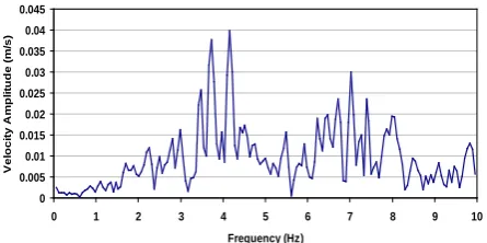
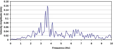
After applying of earthquake acceleration to the silo models, the velocity response of a point at the top of silo in direction of applying earthquake excitation is obtained in frequency domain by FFT (Fast Fourier Transform). The FFT amplitudes of velocity for the silo models are plotted in Figures 5-7. As shown in Figure 5, the frequency corresponding to the highest peak of velocity amplitude in model 1 is 4.15 Hz. There is another peak with frequency of 3.723 Hz, while the computed frequency value by applying 80 percent of granular material mass to the silo wall is 7.394 Hz. The velocity response of model 2 in frequency domain is plotted in Figure 6. As shown in this figure, the frequency corresponding to the highest peak of velocity amplitude in model 2 is 3.662 Hz. However, the computed frequency value by applying 80 percent of granular material mass to the silo wall is 4.9 Hz. The velocity response of model 3 in frequency domain is plotted in Figure 7. As shown in this figure, the frequency corresponding to the highest peak of velocity amplitude in model 3 is 2.319 Hz, while the computed frequency value by applying 80 percent of granular material mass to the silo wall is 2.637 Hz. The results show that the dominant frequency of models with height to diameter ratios of 1 and 2 has much difference with the frequency of first translational mode by considering of 80 percent of granular material mass as effective mass. Nevertheless, in the silo with height to diameter ratio equal to 5 these frequencies have smaller difference.

0 0.005 0.01 0.015 0.02 0.025 0.03 0.035 0.04 0.045

0 1 2 3 4 5 6 7 8 9 10

Frequency (Hz)

V

e

lo

c

it

y

A

m

p

lit

u

d

e

(

m

/s

)

Figure 5. Velocity response of a point at the top of silo

(7)

0 0.02 0.04 0.06 0.08 0.1 0.12 0.14 0.16 0.18

0 1 2 3 4 5 6 7 8 9 10 Frequency (Hz)

V

e

lo

c

it

y

A

m

p

lit

u

d

e

(

m

/s

)

Figure 6. Velocity response of a point at the top of silo in frequency domain in model 2

0 0.2 0.4 0.6 0.8 1 1.2

0 1 2 3 4 5 6 7 8 9 10

Frequency (Hz)

V

e

lo

c

it

y

A

m

p

lit

u

d

e

(

m

/s

)

Figure 7. Velocity response of a point at the top of silo

in frequency domain in model 3

7. DETERMINATION OF FREQUENCY BY CONSIDERING ELASTIC BEHAVIOR FOR GRANULAR

MATERIAL

TABLE 5. Assumed values of modulus of elasticity for

each layer of granular material

Modulus of elasticity (MPa)

Model 1 Model 2 Model 3

Layer 1 15 20 30

Layer 2 40 80 90

Layer 3 90 140 130

Layer 4 130 180 150

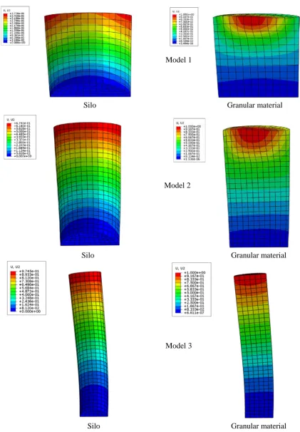
The deformed shapes of silo and granular material inside silo in the first translational mode computed by considering four layers of granular material with elastic behavior are presented in Figure 8 for all models. As shown in Figure 8, in model 1 that has the lowest value of height to diameter ratio, the largest displacements in the first mode have occurred in the first layer of granular material near the top surface of granular material. In model 2 with height to diameter ratio equal to 2 still the largest displacements in the first mode have occurred in the first layer of granular material near the top surface of granular material. But, the difference between largest displacements in silo wall and first layer of granular material is less than the corresponding difference in model 1. In model 3, with height to diameter ratio equal to 5, the difference between largest displacements in silo wall and first layer of granular material is less than other models. It seems that in models with lower higher pressures existing in granular material the

By moving from top to the bottom of silo due to tangential stiffness components in three directions. judgment based on mean of three values of elasticity for these layers were determined by of modulus of elasticity. The values of modulus of was divided into four layers with different values frequency. In each silo model granular material analysis was performed for computation of silo considered to behave elastically and eigenvalue excitation, the granular material inside silo was obtained from the silo response under earthquake material mass as effective mass and frequency computed by considering 80 percent of granular the reason of difference between silo frequency during earthquake excitation. For understanding granular material in each integration point changes incrementally nonlinear and the stiffness of behavior of granular material inside silo is model with intergranular strain extension the In fact by using von Wolffersdorff’s hypoplastic

as effective mass.

(8)

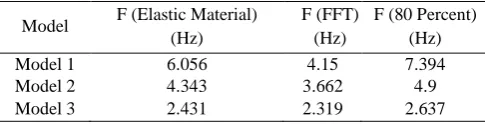
height to diameter ratios due to higher stiffness of silo structure the dominant frequency obtained from FFT of the response is dependent on the stiffness of granular material. In models 1 and 2 that the silo structure is stiffer, the stiffness of granular material in parts near the top surface of granular material has a significant participation in the dominant frequency of response. As shown in Table 6, the computed values of frequency by considering four layers of granular material with elastic behavior in models 1 and 2 still have much difference with the values of dominant frequency obtained from FFT. The reason is that the value of modulus of elasticity assigned to the first layer of granular material overestimates the stiffness value for the part of granular material which is situated near the surface of granular material inside silo. In model 3, the value of dominant frequency obtained from FFT of the response has good correlation with the value of frequency obtained from eigenvalue analysis by considering four layers of granular material with elastic behavior. The reason is that in model 3 which is a slender silo due to flexibility of silo structure, the stiffness of granular material does not have a significant participation in the dominant frequency of response.

TABLE 6. The values of frequency computed by

different methods

Model F (Elastic Material)

(Hz)

F (FFT) (Hz)

F (80 Percent) (Hz)

Model 1 6.056 4.15 7.394

Model 2 4.343 3.662 4.9

Model 3 2.431 2.319 2.637

8. ENVELOPES OF DYNAMIC PRESSURE

The envelopes of dynamic pressure in direction of earthquake excitation for right and left sides of silos are plotted versus height in Figures 9-11 for all models. For obtaining the envelopes of dynamic pressure, at first the time history of dynamic pressure at each node is calculated, for this purpose the time history of contact pressure is subtracted from the value of contact pressure at the end of gravity step. Then, the maximum value of dynamic pressure at each node is considered as the envelope value of dynamic pressure. The envelopes of dynamic pressure are compared with the pressure distribution proposed by Eurocode 8 part 4 [3]. For

calculation of Eurocode pressure distribution α( )z is considered constant. α( )z is obtained from 5 percent damped spectrum of Eurocode 8 [12] for soil type B and design ground acceleration of 0.2g with assuming period computed by considering 80 percent of granular material mass as effective mass. Figure 9 shows the envelopes of dynamic pressure in model 1. As illustrated in this figure, except in the lowest part of silo wall, the envelope values of dynamic pressure are lower than the proposed pressure by Eurocode. Therefore, it can be concluded that assuming a constant value for

( )z

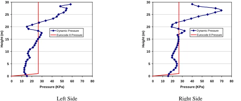
α in squat silos is a rational assumption. Figure 10 shows the envelopes of dynamic pressure in model 2. As illustrated in this figure, in addition to the lowest part of silo wall in few points at the upper half of silo height, the envelope values of dynamic pressure have exceeded the proposed pressure by Eurocode. Figure 11 shows the envelopes of dynamic pressure in model 3. As illustrated in this figure, the envelope values of dynamic pressure have considerably exceeded the proposed pressure by Eurocode at the upper half of silo height. Therefore, it can be concluded that due to impact of granular material into the silo wall assuming a constant value for α( )z in a slender silo is not a conservative assumption.

9. CONCLUSIONS

In slender silo with height to diameter ratio equal to 5, the values of frequency computed by all methods are near each other. However, in silos with lower height to diameter ratios the differences between frequencies computed by different methods are significant. It can be concluded that in silos with lower height to diameter ratios, the vibration of granular material inside silo in parts situated near the top surface of granular material plays an important role in the dominant frequency of response. The stiffness of granular material situated in layers near the top surface of granular material controls the dominant frequency of response.

(9)

Model 1

Silo Granular material

Model 2

Model 3

(10)

0 1 2 3 4 5 6 7 8 9 10

0 10 20 30 40 50

Pressure (KPa)

H

e

ig

h

t (m

)

Dynamic Pressure Eurocode 8 Pressure

0 1 2 3 4 5 6 7 8 9 10

0 10 20 30 40 50

Pressure (KPa)

H

e

ig

h

t (m

)

0 2 4 6 8 10 12 14 16 18 20

0 10 20 30 40 50 60

Pressure (KPa)

H

e

ig

h

t (m

)

0 2 4 6 8 10 12 14 16 18 20

0 10 20 30 40 50 60

Pressure (KPa)

H

e

ig

h

t (m

)

0 5 10 15 20 25 30

0 10 20 30 40 50 60 70 80

Pressure (KPa)

H

e

ig

h

t (m

) Dynamic Pressure Eurocode 8 Pressure

0 5 10 15 20 25 30

0 10 20 30 40 50 60 70 80

Pressure (KPa)

H

e

ig

h

t (m

) Dynamic Pressure Eurocode 8 Pressure

Left Side Right Side

Figure 9. The distribution of dynamic pressure envelopes versus height in direction of earthquake excitation for right and left sides of silo in model 1

Figure 10. The distribution of dynamic pressure envelopes versus height in direction of earthquake excitation for right and left sides of silo in model 2

(11)

in model with height to diameter ratio equal to 2, the envelope values of dynamic pressure in few points at the upper half of silo height have marginally exceeded the Eurocode pressure calculated assuming a constant value for α( )z . Nevertheless, when the height to diameter ratio increases to 5, the envelope values of dynamic pressure at the upper half of silo height have considerably exceeded the Eurocode pressure calculated assuming a constant value for α( )z . It can be due to impact of granular material into the silo wall. Therefore, it can be concluded that considering a constant value for α( )z in a slender silo is not a conservative assumption.