Optimal Pareto Parametric Analysis of Two Dimensional Steady-State Heat Conduction Problems by MLPG Method

(1)

OPTIMAL PARETO PARAMETRIC ANALYSIS OF TWO

DIMENSIONAL STEADY-STATE

HEAT CONDUCTION

PROBLEMS BY MLPG METHOD

G.H. Baradaran

Department of Mechanics, Shahid Bahonar University P.O. Box 76175-133, Kerman, Iran

[email protected]

M.J. Mahmoodabadi*

Department of Mechanics, Guilan University P.O. Box 3756, Rasht, Iran

[email protected]

*Corresponding Author

(Received: January 10, 2009 – Accepted in Revised Form: July 2, 2009)

Abstract Numerical solutions obtained by the Meshless Local Petrov-Galerkin (MLPG) method are presented for two dimensional steady-state heat conduction problems. The MLPG method is a truly meshless approach, and neither the nodal connectivity nor the background mesh is required for solving the initial-boundary-value problem. The penalty method is adopted to efficiently enforce the essential boundary conditions, the moving least squares approximation is used for interpolation schemes and the Heaviside step function is chosen for test function. As the accuracy and runtime will depend on definition radiuses of the moving least squares approximation and the Heaviside step function; therefore, a genetic algorithm is carried out to determine the optimal values for these radiuses. The results show that the present method is very promising in solving engineering two dimensional steady-state heat conduction problems.

Keywords Meshless Local Petrov-Galerkin, Moving Least Squares, Heaviside Step Function, Heat Conduction, Optimization, Genetic Algorithm

ﻜﭼ

ﻴ

ﻩﺪ

ﻲﻠﺤﻣﺵﻭﺭﻪﺑ،ﻱﺪﻌﺑﻭﺩﻱﺎﻀﻓﺭﺩﺭﺎﮔﺪﻧﺎﻣﺖﻟﺎﺣﻲﻳﺎﻧﺎﺳﺭﺕﺭﺍﺮﺣﻝﺎﻘﺘﻧﺍﻞﺋﺎﺴﻣﻞﻴﻠﺤﺗ،ﻪﻟﺎﻘﻣﻦﻳﺍﺭﺩ

ﻑﻭﺮﺘﭘﻥﺎﻤﻟﺍﻥﻭﺪﺑ

-ﻦﻴﮐﺮﻟﺎﮔ

)

MLPG

(

ﺖﺳﺍﻩﺪﺷﻪﺋﺍﺭﺍ،

.

ﺵﻭﺭ MLPG

ﺍﺮﻳﺯ،ﺖﺳﺍﻲﻌﻗﺍﻭﻥﺎﻤﻟﺍﻥﻭﺪﺑﺵﻭﺭﮏﻳ

ﻱﺍﺮﺑﺎﻬﻨﺗﻪﻧ

ﻝﺍﺮﮕﺘﻧﺍ

ﻩﺩﺎﻔﺘﺳﺍﻲﻧﺎﻤﻟﺍﭻﻴﻫﺯﺍﻒﻴﻌﺿﻡﺮﻓﺯﺍﻱﺮﻴﮔ

ﻲﻤﻧ

ﻥﻭﺭﺩﺖﻬﺟﻪﮑﻠﺑ،ﺪﻨﮐ

ﻩﺩﺍﺩﻲﺑﺎﻳ

ﺰﻴﻧﺎﻫ

ﻥﺎﻤﻟﺍﻪﺑ

ﺩﺭﺍﺪﻧﺯﺎﻴﻧﻪﻟﺎﺴﻣﻪﻨﻣﺍﺩﻱﺪﻨﺑ

.

ﻥﻭﺭﺩﻱﺍﺮﺑﻭﻪﻤﻳﺮﺟﺐﻳﺮﺿﺵﻭﺭﺯﺍ،ﻱﺯﺮﻣﻂﻳﺍﺮﺷﻱﺎﺿﺭﺍﻱﺍﺮﺑ

ﻩﺩﺍﺩﻲﺑﺎﻳ

ﺎﻫ

ﺐﻳﺮﻘﺗﺯﺍ

ﺕﻼﺿﺎﻔﺗﻡﻭﺩ ﻥﺍﻮﺗ

)

MLS

(

ﺖﺳﺍﻩﺪﺷﻩﺩﺎﻔﺘﺳﺍ

.

ﭽﻤﻫ

ﻣﺯﺁﻊﺑﺎﺗ،ﻦﻴﻨ

ﻪﻠﭘﻊﺑﺎﺗ،ﻩﺩﺎﻔﺘﺳﺍﺩﺭﻮﻣﻥﻮ

ﺖﺳﺍﺩﺎﺴﻳﻮﻫﻱ

.

ﺯﺍ

ﻉﺎﻌﺷﻪﮐﺎﺠﻧﺁ

ﺐﻳﺮﻘﺗﻊﺑﺎﺗﻭﺩ ﻱﺎﻫ

MLS

ﺏﺍﻮﺟﺖﻗﺩ ﻭﻪﻣﺎﻧﺮﺑﻱﺍﺮﺟﺍ ﻥﺎﻣﺯﻱﻭﺭ ﺮﺑ،ﺪﻳﺎﺴﻳﻮﻫ ﻪﻠﭘﻭ

ﻲﻣﺮﺛﺍ ﺎﻫ

ﻪﻨﻴﻬﺑﺮﻳﺩﺎﻘﻣﻦﻴﻴﻌﺗﻱﺍﺮﺑﻪﻟﺎﻘﻣﻦﻳﺍﺭﺩﻦﻳﺍﺮﺑﺎﻨﺑ،ﺩﺭﺍﺬﮔ

ﻉﺎﻌﺷﻦﻳﺍ

ﺖﺳﺍﻩﺪﺷﻩﺩﺎﻔﺘﺳﺍﮏﻴﺘﻧﮊﻢﺘﻳﺭﻮﮕﻟﺍﺯﺍ،ﺎﻫ

.

ﻪﺴﻳﺎﻘﻣ

ﺻﺎﺣﺞﻳﺎﺘﻧ

ﺭﺎﮔﺪﻧﺎﻣﺖﻟﺎﺣﻲﻳﺎﻧﺎﺳﺭﺕﺭﺍﺮﺣﻝﺎﻘﺘﻧﺍﻞﺋﺎﺴﻣﻞﻴﻠﺤﺗﺭﺩﺵﻭﺭﻦﻳﺍﺖﻴﻘﻓﻮﻣﺮﮕﻧﺎﻴﺑ،ﻖﻴﻗﺩﻱﺎﻫﺏﺍﻮﺟﺎﺑﻞ

ﺪﺷﺎﺑﻲﻣﻱﺪﻌﺑﻭﺩﻱﺎﻀﻓﺭﺩ

.

1. INTRODUCTION

In recent years, the meshless method has emerged as an effective numerical approach to find solutions of initial-boundary-value problems. The MLPG method is one of the meshless schemes. The main advantage of this method compared with other meshless methods is that no background

(2)

elasto-static problems, Lin, et al [2] introduced the up winding scheme to analyze steady state convection-diffusion problems, and Liu, et al [3] coupled the MLPG method with the finite element also with the boundary element method to enhance the efficiency of the MLPG method. Ching, et al [4] augmented the polynomial basis functions with singular fields to determine deformations and stress fields near the crack tip for generally 2D mixed-mode problems. Gu, et al [5] and Batra, et al [6] used the Newmark family of methods to analyze 2D transient elastodynamic problems. The bending of a thin plate has been studied by Gu, et al [7] and Long, et al [8]. The objective of this work is to present the MLPG analysis for two dimensional steady-state heat conduction problems. First, we list governing equations next, the weak formulations of MLPG method and the moving least squares (MLS) approximation is briefly introduced.

MLPG and other meshless methods have several parameters that have to be chosen correctly to achieve good accuracy. A Genetic Algorithm (GA) is a computational model that emulates biological evolutionary theories to solve optimization problems. In this paper, multi-objective GA is used to optimal Pareto parametric analysis for two dimensional steady-state heat conduction. It should be noted that there are many different ways of hybridization; but most of them incorporate a local optimizer to the simple GA main loop. Further, a new method called ε-elimination diversity algorithm, recently proposed [9,10] that this algorithm is used in this article too.

Four examples are analyzed to demonstrate the validity and versatility of the method. The results obtained are in good agreement with the analytical solutions.

2. MLPG FORMULATION

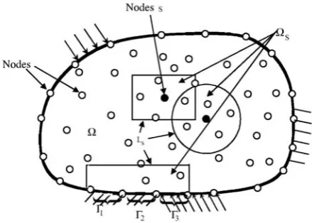
We consider a 2D heat conduction problem, as shown in Figure 1, for illustrating the procedure for formulating the MLPG method. The problem domain is denoted by Ω, which is bounded by boundaries including essential boundary Γ1, natural

boundary Γ2 and Robin boundary Γ3. In the MLPG

method, the problem domain is represented by a

set of arbitrarily distributed nodes, as shown in same. The weighted residual method is used to create the discrete system equation.

The major idea in MLPG is that the implementation of the integral form of the weighted residual method is confined to a very small local sub domain of a node. This means that the weak form is satisfied at each node in the problem domain in a local integral sense. Therefore, the weak form is integrated over a "local quadrature domain" that is independent of other domains of other nodes. This is made possible by use of the Petrov-Galerkin formulation, in which one has the freedom to choose the test and trial functions independently.

The heat conduction Poisson’ equation and boundary conditions can be written as:

Ω ψ = θ + θ

λ ₂) in

dy 2 d 2 dx

2 d

( & (1)

The Dirichlet boundary condition:

1 on

1 Γ

θ =

θ (2)

The Neumann boundary condition:

2 on q ) y n dy d x n dx d

( θ + θ = Γ

λ

− (3)

The Robin boundary condition:

3 on ) f ( h ) y n dy d x n dx d

( θ + θ = θ −θ Γ

λ (4)

(3)

Where θ represents temperature; λ the thermal conductivity, nx and ny are the component the

outward unit vector to Γ, q the given heat flux, h the convection heat transfer coefficient, θf is the

environmental temperature, ψ& the heat source per unit mass, and Γ1, Γ2 and Γ3 the boundaries at

which the Dirichlet, Neumann and Robin conditions apply, respectively.

In the Ωs, the weighted integral form of

Equation 1 is given as

0 s d s ) 2 dy 2 d 2 dx 2 d

( υ Ω =

∫ Ω ⎥ ⎥ ⎦ ⎤ ⎢ ⎢ ⎣ ⎡ ψ − θ + θ

λ & (5)

In Equation 5 υ is test function. To reduce this high-order differentiability requirement on θ, we can integrate Equation 5 by parts. By using Gauss’s theorem, we can obtain the following local weak formulation equation:

0 s dL s L y n dy d x n dx d 1 d 1 y n dy d x n dx d s d s dy d dy d dx d dx d =

∫ _⎟⎟υ

⎠ ⎞ ⎜⎜

⎝

⎛ θ ₊ θ

λ − Γ ∫ Γ υ ⎟⎟ ⎠ ⎞ ⎜⎜ ⎝

⎛ θ ₊ θ

λ −

Ω ∫

Ω ⎟⎟⎠

⎞ ⎜⎜ ⎝ ⎛ υ ψ + υ θ λ + υ θ λ & (6)

In this equation Ls being the other part of the local

boundary which is inside the solution domain. Substituting Equation 3 and Equation 4 into Equation 6, we can obtain Equation 7.

0 s dL s L y n dy d x n dx d 1 d 1 y n dy d x n dx d 3 d 3 ) f ( h 2 d 2 q s d s dy d dy d dx d dx d =

∫ _⎟⎟υ

⎠ ⎞ ⎜⎜

⎝

⎛ θ ₊ θ λ − Γ ∫ Γ υ ⎟⎟ ⎠ ⎞ ⎜⎜ ⎝ ⎛ θ + θ λ − Γ ∫ Γ υ θ − θ − Γ ∫ Γ υ + Ω ∫

Ω ⎟⎟⎠

⎞ ⎜⎜ ⎝ ⎛ υ ψ + υ θ λ + υ θ λ & (7)

The MLS approximation function is given by

∑ = ∧ θ φ = θ N 1 I I I

(8)

Here, θˆ is the unknown fictitious nodal values and ØI is usually called as the shape function of MLS

approximation corresponding to nodal point SI.

Substitution of Equation 7 into Equation 8 for all the nodes, we can obtain the following linear equations:

1 d 1 I 1 3 d I f h 3 2 d 2 I q s d s I M 1 J 1 d 1 I J J M 1 J s dL s

L y I

n dy J J d x n dx J J d M 1 J 1 d 1 I y n dy J J d x n dx J J d M 1 J 3 d 3 I J J h M 1 J s d s dy I d dy J J d dx I d dx J J d Γ ∫ Γ θυ α + Γ υ θ ∫ Γ + Γ ∫ Γ υ − Ω ∫ Ωψυ − = ∑

= Γ∫ υ Γ

∧ θ φ α + ∑

= ∫ _⎟⎟υ

⎟ ⎟ ⎠ ⎞ ⎜ ⎜ ⎜ ⎜ ⎝ ⎛ ∧ θ φ + ∧ θ φ λ − ∑

= Γ∫ _⎟⎟υ Γ

⎟ ⎟ ⎠ ⎞ ⎜ ⎜ ⎜ ⎜ ⎝ ⎛ ∧ θ φ + ∧ θ φ λ − ∑

= Γ∫ Γ

υ ∧ θ φ + ∑

= Ω∫ _⎟⎟ Ω

⎟ ⎟ ⎠ ⎞ ⎜ ⎜ ⎜ ⎜ ⎝ ⎛ υ ∧ θ φ λ + υ ∧ θ φ λ & (9)

In Equation 9 M is the total number of nodes in the entire domain Ω, or

F θ

K.∧= (10)

In Equation 10 θˆ _{the vector for the unknown} fictitious nodal values, α the penalty parameter, which is used to impose the essential boundary conditions, and K and F are the global stiffness matrix and the global vector, respectively, which are defined as

1 d 1 I J s L d s

L y I

n dy J d x n dx J d 1 d 1 I y n dy J d x n dx J d 3 d 3 I J h s d s dy I d dy J d dx I d dx J d IJ K Γ ∫ Γ υ φ α +

∫ _⎟⎟υ

⎠ ⎞ ⎜ ⎜ ⎝ ⎛ _φ + φ λ − Γ ∫ Γ υ ⎟ ⎟ ⎠ ⎞ ⎜ ⎜ ⎝ ⎛ _φ + φ λ − Γ ∫ Γ υ φ + Ω ∫ Ω ⎟ ⎟ ⎠ ⎞ ⎜ ⎜ ⎝

⎛ _φ υ

(4)

1 d 1

I 1 3

d I f h 3

2 d 2

I q s d s

I I

F

Γ ∫

Γ υ θ α + Γ υ θ ∫ Γ +

Γ ∫ Γ

υ − Ω ∫ Ω

υ ψ − = &

(12)

In MLPG shape functions do not satisfy the Kronecker delta property, and hence when such trial functions are used, it is not easy to implement the essential boundary.

Various numerical techniques have been proposed to enforce the essential boundary conditions, such as the Lagrange multiplier method, the penalty approach, the transformation method, the direct interpolation method, etc. In the present work, the penalty approach has been used to enforce essential boundary conditions.

Because discretization errors can be comparable in magnitude to the errors due to the poor satisfaction of the constraint, the following formula has been suggested for determining the penalty parameter in FEM analysis [11]:

n h 1

const ⎟

⎠ ⎞ ⎜ ⎝ ⎛ × =

α (13)

Where h is the characteristic length, which can be the ratio of the element size to the dimension of the problem domain, and n is the order of the elements. In extending this formula to meshless methods, we suggest that h be the ratio of the nodal spacing to the dimension of the problem domain, and n = 1. The constant in Equation 13 should relate to the material property of the solid or structure. It can be 1010_{times Young's modulus.}

This paper prefers the following simple method for determining the penalty parameter:

K) in elements diagonal

(max

β

10

α= × 4≤β≤18 (14)

In Equation 14 K is the global stiffness matrix. In most of the examples reported using penalty methods, the foregoing equation is adopted. It has also been suggested to use

modulus) (Young

β

10

α= × 5≤β≤8 (15)

Equation 15 works well in elasto-static problems. Note that trials may be needed to choose a proper penalty parameter.

3. THE MOVING LEAST SQUARE APPROXIMATION SCHEME

Moving Least Squares (MLS), originated by mathematicians for data fitting and surface construction, can be categorized as a method of finite series representation of functions. The MLS method is now a widely used alternative for constructing meshless shape functions for approximation.

The MLS approximation has two major features that make it popular: (1) the approximated field function is continuous and smooth in the entire problem domain; and (2) it is capable of producing an approximation with the desired order of consistency. The MLS approximation is detailed in this part.

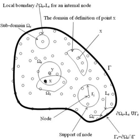
Consider a support domain Ωx, which is located

within the problem domain Ω (Figure 2) and has a number of randomly located nodes xI (I = 1,...,N).

The moving least squares approximate θh_{(x) of}

θ(x) by following definition:

) x ( i a ) x ( m

1 i pi )

x (

h _∑

= =

θ = pT_{(x) a(x)} ₍₁₆₎

Where pT_(x)=[p

1(x),p2(x),...,pm(x)] is a complete

monomial basis, m is the number of terms in the basis, and a(x)=[a1(x),a2(x),...,am(x)] is the

(5)

corresponding coefficient. For example, for a 2D problem, the basis can be chosen as

] 2 y xy, , 2 x y, x, [1, (x) T p : 6) (m basis Quadratic y] x, [1, (x) T p : 3) (m basis Linear = = = = (17)

The coefficient vector a(x) is determined by minimizing the difference between the local approximation and the function, and is defined as

( )

(

)

( )

x θˆ]TW[Pa

( )

x θˆ] Pa [ 2 N 1 I I θˆ x a I x T P x I w x a J − − = ∑ = ⎥⎦ ⎤ ⎢⎣ ⎡ _⎟ ₋ ⎠ ⎞ ⎜ ⎝ ⎛

= ₍₁₈₎

Where xI denotes the position vector of node I,

wI(x) is the weight function associated with the

node I, N is the number of node in Ωx for which

the weight functions wI(x) > 0 are searched, the

matrix P and the diagonal matrix W are defined as

m N ) N (x m p ... ) N (x 2 p ) N (x 1 p . . . ) 1 (x m p ... ) 2 (x 2 p ) 2 (x 1 p ) 1 (x m p ... ) 1 (x 2 p ) 1 (x 1 p P × ⎥ ⎥ ⎥ ⎥ ⎥ ⎥ ⎥ ⎦ ⎤ ⎢ ⎢ ⎢ ⎢ ⎢ ⎢ ⎢ ⎣ ⎡

= (19)

( )

N N x N w . . . 0 . . . . . . . . . 0 . . . x 1 w W × ⎥ ⎥ ⎥ ⎥ ⎥ ⎥ ⎦ ⎤ ⎢ ⎢ ⎢ ⎢ ⎢ ⎢ ⎣ ⎡

= (20)

and N 1 N θˆ ,..., 2 θˆ , 1 θˆ T θˆ × ⎥⎦ ⎤ ⎢⎣ ⎡

= (21)

In Equation 21 θ∧I is the fictitious nodal value. It is not the nodal value of trial functions denoted by θh_(x).

To find the coefficient a(x), we obtain the extremum by 0 ) I (x i p N 1 I m 1 i I θˆ )a(x) I (x i p (x) I w 2 (a(x)) J(a(x)) = ∑ = ⎥⎥⎦ ⎤ ⎢ ⎢ ⎣ ⎡ ∑ = − = ∂ ∂ (22)

This leads to the following set of linear relations:

( ) ( ) ( )

(

m m

)(

m 1

) (

m N

)(

N 1

)

θˆ x B x a x A × × = × × = ₍₂₃₎

Where the matrixes A(x) and B(x) are defined by

( ) ( ) ∑ ( ) = ⎟⎠ ⎞ ⎜ ⎝ ⎛ ⎟ ⎠ ⎞ ⎜ ⎝ ⎛ = = = N 1

I xI

T p I x p x I w P x B WP T P x

A (24)

( )

_⎥⎦⎤ ⎢⎣ ⎡ _⎟ ⎠ ⎞ ⎜ ⎝ ⎛ ⎟ ⎠ ⎞ ⎜ ⎝ ⎛ ⎟ ⎠ ⎞ ⎜ ⎝ ⎛ = = N x p x N w ,..., 2 x p x 2 w , 1 x p x 1 w W T P x B (25)

Solving a(x) from Equation 23, and substituting it into Equation 16, we can obtain the final form of the MLS approximation as

( )

x Ω x , I θˆ I θ I x h θ N 1 I I θˆ x I φ θˆ x T Φ x h θ ∈ ≠ = ⎟ ⎠ ⎞ ⎜ ⎝ ⎛ ∑ = = = (26)

Where ФT_{(x) = p}T_(x)A-1_{(x)B(x) is the shape}

function, and its partial derivative is:

∑ = _⎥⎥ ⎥ ⎥ ⎦ ⎤ ⎢ ⎢ ⎢ ⎢ ⎣ ⎡ ⎟ ⎠ ⎞ ⎜ ⎝ ⎛ − ₊ − + ⎟ ⎠ ⎞ ⎜ ⎝ ⎛ − = m 1 j jI B 1 K , A K , B 1 A j p jI B 1 A k j, p I K ,

φ (27)

In practical applications, the weight function wI(x)

is generally nonzero over the small neighborhood of point xI, and this neighborhood is called the

domain of influence or the domain of definition (Figure 2). Typically, the shape of the domain in the two dimensional space can be circular, ellipse, rectangular or any other convenient regular closed lines and in the three dimensional space can be sphere, ellipsoid, cube or any other simple cubic volume. In the present analysis a circular domain has been selected. The choice of weight function wI(x) affects the resulting approximation θh(x);

(6)

⎪ ⎪ ⎪ ⎩ ⎪ ⎪ ⎪ ⎨ ⎧

≥ ≤ ≤ ⎟ ⎟ ⎠ ⎞ ⎜ ⎜ ⎝ ⎛ − ⎟ ⎟ ⎠ ⎞ ⎜ ⎜ ⎝ ⎛ + ⎟ ⎟ ⎠ ⎞ ⎜ ⎜ ⎝ ⎛ − =

I r I d 0

I r I d 0 4

I rI d 3 3

I rI d 8 2

I rI d 6 1

) X ( I

w (28)

Where dI is the distance between points x and nod

xI and rI is the size of support (Figure 2) for the

weight functions. It can be seen that the quadratic spline weight function is C1 continuous over the entire domain.

4. GENETIC ALGORITHMS-HOW AND WHY?

4.1. Genetic Algorithm Basics

A Genetic

Algorithm (GA) is a computational model that emulates biological evolutionary theories to solve optimization problems. A GA is a technique used to automate the process of searching for an optimal solution. Because it searches from a population of points, the probability of the searches getting trapped in a local minimum is limited. GAs start searching by randomly sampling within an optimization solution space, and then use stochastic operators to direct a process based on objective function values.

UnderGA terminology, a solution to a problem is an individual and a group of individuals is a population. A generation is a new population. In binary GAs, each individual is represented by a binary string called a chromosome, which encodes all the parameters of interest corresponding to that individual. A chromosome is formed of alleles, the binary coding bits. The fitness of any particular individual corresponds to the value of its objective function.

Genetic operators control the evolution of successive generations. The three basic genetic operators are reproduction, crossover and mutation. The probability of a given solution’s being chosen for reproduction is proportional to the fitness of that solution. Crossover implies that parts of two randomly chosen chromosomes will be swapped to create a new individual. Mutation involves randomly changing an allele in a solution to look for new points in the solution space.

Although there are more elaborate versions of these operators, the basic principles remain similar for most GAs.

A genetic algorithm starts by generating a number of possible solutions to a problem, evaluates them and applies the basic genetic operators to that initial population according to the individual fitness of each individual. This process generates a new population with higher average fitness than the previous one, which in turn will be evaluated. The cycle is repeated for the number of generations set by the user, which is dependent on problem complexity.

4.2. Why Use A GA?

GAs offer several attractive features:

• An easily understood approach that can be applied to a wide range of problems with little or no modification. Other approaches have required substantial alteration to be successfully used in building applications. For example, dynamic programming was applied to the problem of selecting the number, location, and power of lamps along a hallway to minimize the electrical power needed to produce the required illuminance [12]. Because the choice of the location and power of a lamp affected decisions made about previous lamps, the sequential decision-making approach inherent in dynamic programming could not be made. It was necessary to suspend earlier decisions and reconsider them, substantially increasing computation time and data storage.

• Publicly available, easily implemented GA codes. Reduced set-up time makes them attractive relative to other optimization methods that may offer better performance but must be identified, obtained and properly configured.

• Inherent capability to work with complex simulation programs. Simulation does not need to be simplified to accommodate optimization.

(7)

minima that would potentially trap a gradient-based method [13]. Building optimization problems may include a mixture of a large number of integer and continuous variables, non-linear inequality and equality constraints, a discontinuous objective function and variables embedded in constraints but not in the objective function. Such characteristics make gradient-based optimization methods inappropriate and restrict the applicability of direct-search methods [14]. The calculation time of mixed integer programming (MIP), which was used to optimize the operation of a district heating and cooling plant, increases exponentially with the number of integer variables. It was shown to take about two timeslongerthan aGA for a 14 hr optimization window and 12 times longer for a 24 hr period [15], although the time required by MIP was sufficiently fast for a relatively simple plant to make on-line use feasible. • Methods to permit GAs to handle constraints

that would make some solutions unattractive or entirely infeasible.

• Identification of optimal trade-offs among multiple optimization criteria, a topic to be discussed next.

4.3. Multi-Objective Optimization

Single-objective optimization may unnecessarily constrain a designer. For example, operating costs for lights and for space conditioning can both be expressed in the same units, but a designer may have reason to favor day lighting from north-facing windows over increased conduction losses and attendant increases in heating and cooling costs. Capital costs for equipment and the building envelope can in principle be included in a life-cycle-cost objective function but may better be considered separately, if capital and operating budgets are separate. Multi-criteria optimization methods move away from a sum (weighted or unweighted) of individual objectives and provide the designer with explicit information about the trade-offs between different criteria.

There are several approaches to multi-objective optimization problems using GAs:

• Simple aggregation or weighting of individual objectives;

• Population based non Pareto approaches;

• Pareto-based approaches.

4.4. Simple Aggregation

Individual objective functions can be combined by using weighting factors based on some knowledge of the problem, forming a single figure of merit that reflects the overall performance of the solution according to the different objectives. Then GAs can be applied repetitively, if necessary, changing the values of the weighting factors at each run, to gain some insight into the relative importance of each of the objectives.

4.5. Population Based Non Pareto Approaches

These approaches seek to discover multiple non-dominated solutions, but without explicit use of Pareto fitness. The Vector Evaluated GA (VEGA) [16] selects sub populations of the next generation according to individual objectives. Overall fitness is a linear combination of individual objectives, with weights that depend on population distributions. Fourman [17] selected a new population by comparing pairs of individuals, each according to one of the objectives.

4.6. Pareto Based Approaches

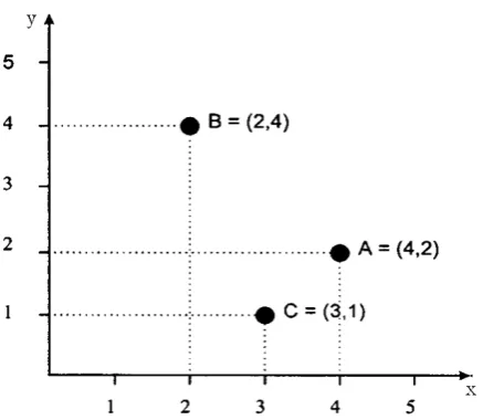
Pareto optimality makes use of the concept of dominated and non-dominated solutions. A solution is Pareto optimal if it is not dominated by any other solution. In Figure 3, the points represent feasible solutions to a multi-objective maximization problem, where values for each of two objective functions are assigned to the x and y axes. A solution dominates another if it is better than the other for at least one objective function and at least as good on all the others [18]. Point A(4,2) dominates point C(3,1) because it has both higher x and y values. Points A(4,2) and B(2,4) are not dominated and are therefore both Pareto-optimal solutions. They represent good trade-offs between the two objective functions. Point A performs better than B in terms of the x values but the inverse is true for y values. There are several Pareto approaches to evolving a population that optimizes the trade-offs among objective functions:

(8)

• Tournament selection [20]. The best of a randomly chosen subset of individuals is chosen for the next generation.

• Pareto reservation strategy [21]. All non-dominated individuals in a population are retained. If necessary to fill out the population of the next generation, remaining individuals are selected via a VEGA.

• Pareto-optimal selection method. All non-dominated individuals in a population are retained and all dominated individuals are discarded.

• Non-dominated Sorting Genetic Algorithm (NSGA) [22].

Niche-induction techniques are used to spread the population of Pareto-optimal solutions over the entire Pareto front.

Crowding and fitness sharing have been used to maintain genetic diversity. GAs is well suited for generating a Pareto front because they work with a population of solutions. Simulated annealing, an optimization that offers many of the advantages of GAs but typically works with a single solution and single objective function, has also been used for multi-objective problems, by archiving non-dominated solutions. On a GA comprise a set of individual elements (the population) and a set of biologically inspired operators defined over the population itself. According to evolutionary

theories, only the most suited elements in a population are likely to survive and generate offspring, thus transmitting their biological heredity to new generations.

4.7. Multi-Objective Optimization of MLPG

Analysis

The vector [r,r0], is the vector of

selective parameters of MLPG analysis. r is support domain radius and r0 is sub domain radius.

The amount of runtime and error of the analysis, are functions of this vector’s components. This means that by selecting various values for the selective parameters, we can make changes in the amounts of runtime and error of MLPG analysis. In this paper we are concerned in choosing values for the selective parameters to minimize above two functions. Clearly this is an optimization problem with two object functions (runtime and error) and two decision variables (r,r0).To solve this problem, we can make use of

single-objective optimization (SOO) or multi-objective optimization (MO) algorithms.

When using SOO, we must exchange the multiple objective functions into one (using weight coefficients). Designer must decide about weight coefficients for all objective functions in proportion to optimality importance of each one of them. So the algorithm returns a single answer corresponding to weight coefficients. As compared with SOO, MO’s results are more complete and flexible. MO in a single run returns a Pareto set of answers which includes all SOO’s answers too. A Pareto set is a set of predominant answers which are non-dominated to each other (don’t have Pareto dominance to each other). This means we can’t find two members of this set that one is better than the other respect to all of objective functions. A Pareto set of answers presents possible different states to which optimal answers can achieve with respect to their objective functions. It shows the condition of confrontation among objective functions and how they vary from answer to answer. As a result, designers by considering the interaction among objective functions can haggle over optimality of them. So they can select an optimum and multipurpose answer consciously. In this paper we used MO to find the selective parameters.

The aim of optimization in this section is finding the selective parameters of MLPG analysis

(9)

in to minimize the error and runtime of analysis. Constraint considered in the analysis is non singularity of total stiffness matrix. To do this Constraint, objective functions of design vectors which break the constraints are set as infinity, to be removed from the cycle in evolution process.

5. RESULTS OF NUMERICAL EXAMPLES

In this section the meshless local Petrov-Galerkin method is applied to compute two dimensional steady-state heat conduction problems. Results of four examples are compared with analytical solution.

We used 6 Gauss points for numerical evaluation of line integrals and a 4 × 4 quadrature scheme (i.e., 16 Gauss points) to evaluate domain integrals. As the accuracy of the result and the time of the run are the effective by the choice of radiuses of the moving least squares approximation and the Heaviside step function, a parametric study is carried out on these parameters that are r and r0.

The influence of the parameters on as the accuracy of the result and the time of the run for several problems is assessed.

A. Example 1

We use these boundary conditions for Poisson’ equation as (see Figure 4)

θ = 0 at x = 0

θ = 0 at x = a

θ = sin(x) at y = 0

θ = 0 at y = b (29)

The analytical solutions for this problem are

) sinh(

) x sin( ) y sinh( y

x

π − π = ) , (

θ (30)

) sinh(

) x cos( ) y sinh( y

x

qx _π

− π λ = ) ,

( (31)

) sinh(

) x sin( ) y cosh( y

x

qy _π

− π λ − = ) ,

( (32)

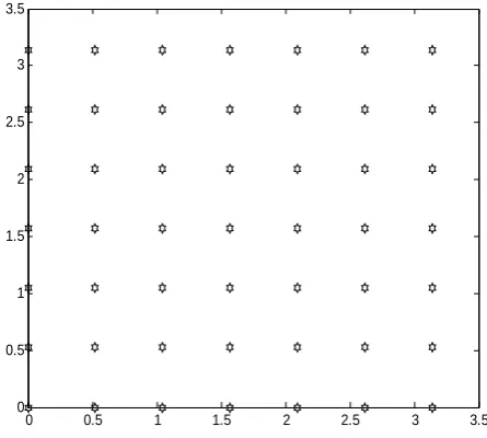
The node distribution with 49 nodes is presented in Figure 5 for the case of a = b = π.

The temperature distributions are presented in Figures 6 and 7. The heat flux distributions are

presented in Figures 8 and 9. The values of r and r0

applied in this example are the same as the values of r and r0 at point C which is shown in Figure 10.

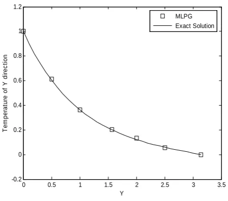
As shown in these figures, the MLPG results agree with the values obtained by analytical solution. The convergence of the MLPG approach is demonstrated in these figures.

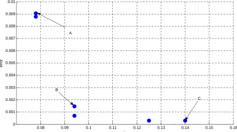
Figure 10 is the chart resulted from multi-objective optimization for the radius of support domain (r) and the radius of sub domain (r0) which

(a,b)

x y

θ=0

θ=sin(x)

ψ

.

=0

λ=50

Figure 4. Geometry and boundary conditions used for example 1.

0 0.5 1 1.5 2 2.5 3 3.5

(10)

all the presented points in they, are non-dominated to each other. Each point in this chart is a representative of a vector of selective parameters which when we choose it for MLPG analysis, the analysis tends to objective functions corresponding to that point of chart.

Values of r and r0 parameters for points A, B

and C, as shown in Figure 10, are given in Table 1.

In this table the r and r0 parameters are normalized

and dimensionless. Results of error and runtime associated with each point are given as well.

Achieving several answers which all of them are considered optimum is a unique property of multi-objective optimization.

B. Example 2

In this case boundary conditions

0 0.5 1 1.5 2 2.5 3 3.5

0 0.02 0.04 0.06 0.08 0.1 0.12 0.14 0.16 0.18 0.2

X

T

e

m

per

at

ur

e

MLPG Exact Solution

Figure 6. Comparison of temperature distribution along 2 y=π.

0 0.5 1 1.5 2 2.5 3 3.5

-0.2 0 0.2 0.4 0.6 0.8 1 1.2

Y

T

e

m

per

at

ur

e of

Y

dir

e

c

tion

MLPG Exact Solution

Figure 7. Comparison of temperature distribution along 2 x=π.

0 0.5 1 1.5 2 2.5 3 3.5

-15 -10 -5 0 5 10 15

X

di

re

c

ti

on H

eat

f

u

x

MLPG Exact Solution

Figure 8. Comparison of heat flux distribution along 2 y= π.

0 0.5 1 1.5 2 2.5 3 3.5

-12 -10 -8 -6 -4 -2 0 2

X

y

dir

e

c

tion H

eat

f

u

x

MLPG Exact Solution

(11)

imposed are presented in Figure 11 as qx = 0 at x = 0

qx = λsin(y) at x = π

θ = 0 at y = 0

θ = 0 at y = π (33) The exact solutions for this problem are

) sinh(

) y sin( ) x cosh( y

x

π =

) , (

θ (34)

) sinh(

) y sin( ) x sinh( y

x q_x

π λ

= ) ,

( (35)

) sinh(

) y cos( ) x cosh( y

x q_y

π λ

= ) ,

( (36)

The node distribution with 100 nodes is presented in Figure 12 for the case of a = b = π.

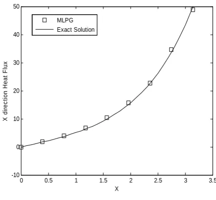
The temperature distribution is presented in Figure 13 and the heat flux distributions are

0.08 0.09 0.1 0.11 0.12 0.13 0.14 0.15 0.16

0 0.001 0.002 0.003 0.004 0.005 0.006 0.007 0.008 0.009 0.01

runtime

er

ror

A

B

C

Figure 10. MO Pareto result for example 1.

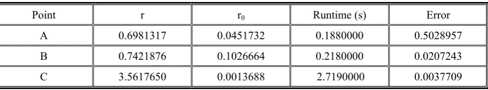
TABLE 1. Comparison Among Points A, B and C for Figure 10.

Point r r0 Runtime (s) Error

A 1.0605140 0.0246399 0.0780000 0.0090746

B 1.3534751 0.0780264 0.0940000 0.0006979

(12)

presented in Figure 14. The values of r and r0

As shown in these figures, the MLPG results agree with the values obtained by analytical solution. The multi-objective optimization results are presented in Figure 15. As shown in this figure, when the error is decrease, the runtime is increase. Values of r and r0 parameters for points A, B

and C, as shown in Figure 15, are given in Table 2. In this table the r and r0 parameters are normalized

Designer in facing to Pareto charts, between several different optimum points can choose a suitable multisided design point easily.

C. Example 3

In this example the MLPG

x

θ

=0

θ

=0

q

_x

=0

q

_x

=

λ

sin(y)

y

(a,b)

ψ

=0

λ

=50

.

0 0.5 1 1.5 2 2.5 3 3.5

Figure 12. Regular node distribution for example 2.

0 0.5 1 1.5 2 2.5 3 3.5

0 0.2 0.4 0.6 0.8 1 1.2 1.4

X

T

e

m

p

er

at

ur

e

MLPG Exact Solution

Figure 13. Comparison of temperature distribution along 2 y= π.

0 0.5 1 1.5 2 2.5 3 3.5

-10 0 10 20 30 40 50

X

di

re

c

ti

on H

eat

F

lux

MLPG Exact Solution

(13)

approach is applied for heat conduction problem with boundary conditions imposed as (see Figure 16)

qx = 0

at x = 0

θ = y2_{at x = a}

qy = 0

at y = 0

θ = x2 at y = b (37)

The analytical solutions for this problem are

θ (x,y) = x2 _{+ y}2 _{- 1} ₍₃₈₎

qx (x,y) = 2λx (39)

qy (x,y) = 2λy (40)

The node distribution with 100 nodes is presented in Figure 17 for the case of a = b = 1.

The temperature distribution is presented in Figure 18 and the heat flux distribution is presented in Figure 19. The values of r and r0

0 0.5 1 1.5 2 2.5 3

0 0.1 0.2 0.3 0.4 0.5 0.6 0.7

runtime

er

ro

r _A

B _C

TABLE 2. Comparison Among Points A, B and C for Figure 15.

A 0.6981317 0.0451732 0.1880000 0.5028957

B 0.7421876 0.1026664 0.2180000 0.0207243

(14)

As shown in this figure, the convergence of the MLPG approach is demonstrated.

Figure 20 is the chart resulted from multi-objective optimization which all the presented points in that are non-dominated to each other. This figure shows the results for this example is alike with the results obtain from previous examples. Values of r and r0 parameters for points A, B

and C, as shown in Figure 20, are given in Table 3.

In this table the r and r0 parameters are normalized

Achieving several answers which all of them are considered optimum is a unique property of multi-objective optimization. Designer in facing to Pareto charts, between several different optimum points can choose a suitable multisided design point easily.

x

θ=x2

q_x=0

y

(a,b)

ψ=100

λ=25

.

q_y=0

θ=y2

0 0.1 0.2 0.3 0.4 0.5 0.6 0.7 0.8 0.9 1

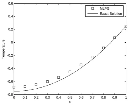
0 0.1 0.2 0.3 0.4 0.5 0.6 0.7 0.8 0.9 1 -0.8

-0.6 -0.4 -0.2 0 0.2 0.4 0.6

X

T

e

m

p

e

rat

ur

e

MLPG Exact Solution

Figure 18. Comparison of temperature distribution along 2 y=1.

0 0.1 0.2 0.3 0.4 0.5 0.6 0.7 0.8 0.9 1 -10

0 10 20 30 40 50

X

dir

e

c

tion H

aet

F

lux

MLPG Exact Solution

(15)

D. Example 4 In this example the MLPG approach

is applied for heat conduction problem with boundary conditions imposed as (see Figure 21)

qx = 0 at x = 0

qx = 0 at x = a

θ = 0 at y = 0

θf = 21 and h = 8 at y = b (41)

The exact solutions for this problem are

θ (x,y) = y2₍₄₂₎

qx (x,y) = 0 (43)

qy (x,y) = 2λy (44)

The node distribution with 100 nodes is presented in Figure 22 for the case of a = b = 1.

The temperature distribution is presented in Figure 23. The heat flux distributions are presented in Figures 24 and 25. The values of r and r0 applied

in this example are the same as the values of r and r0 at point C which is shown in Figure 26. As

shown in these figures, the results agree with the

1.04 1.06 1.08 1.1 1.12 1.14 1.16 1.18 1.2 1.22

0.0475 0.048 0.0485 0.049 0.0495 0.05 0.0505 0.051

runtime

e

rro

r

A

B

C

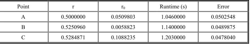
TABLE 3. Comparison Among Points A, B and C for Figure 20.

A 0.5000000 0.0509803 1.0460000 0.0502548

B 0.5250960 0.0058823 1.1400000 0.0489875

(16)

exact solution. The convergence of this approach is demonstrated in these figures.

Each point in Figure 26 is representative of a vector of selective parameters which when we choose them for MLPG analysis, the analysis tends to objective functions corresponding to that point of chart.

Values of r and r0 parameters for points A, B

and C, as shown in Figure 26, are given in Table 4. In this table the r and r0 parameters are normalized

As shown in Table 4 when the support domain (r) increases and the sub domain (r0) decreases then

the runtime increases and the error decreases.

x

q

_x

=0

y

(a,b)

ψ

=160

λ

=80

.

θ

=0

q

_x

=0

θ

_f

=21

h=8

0 0.1 0.2 0.3 0.4 0.5 0.6 0.7 0.8 0.9 1

0 0.1 0.2 0.3 0.4 0.5 0.6 0.7 0.8 0.9 1 -0.2

0 0.2 0.4 0.6 0.8 1 1.2

Y

T

e

m

p

er

a

tur

e

MLPG Exact Solution

Figure 23. Comparison of temperature distribution along

2 x=1.

0 0.1 0.2 0.3 0.4 0.5 0.6 0.7 0.8 0.9 1 0

20 40 60 80 100 120 140 160

Y

y

di

re

c

ti

o

n

H

a

et

F

lux

MLPG Exact Solution

(17)

0 0.1 0.2 0.3 0.4 0.5 0.6 0.7 0.8 0.9 1 -1

-0.8 -0.6 -0.4 -0.2 0 0.2 0.4 0.6 0.8

1x 10

-8

Y

X

d

ir

e

c

ti

on H

a

e

t F

lux

MLPG Exact Solution

Figure 25. Comparison of heat flux distribution along 2 x=1.

1 1.5 2 2.5 3 3.5 4 4.5

0.0335 0.034 0.0345 0.035 0.0355 0.036 0.0365 0.037

runtime

er

ror

A

B

C

(18)

6. CONCLUSION

The meshless local Petrov-Galerkin (MLPG) method that uses a Heaviside test function is presented and used to analyze heat conduction problems. By using a Heaviside test function, the domain integral in the weak form is simplified. This substantially reduces the computation effort to construct the stiffness matrix and hence is computationally efficient compared to the conventional MLPG method. The penalty approach is used to impose the essential boundary conditions and the moving least squares approximation is used for interpolation schemes. A genetic algorithm is carried out to determine the optimal values for

definition radiuses of the moving least squares approximation and the Heaviside step function. The present results show that the MLPG algorithm with a Heaviside test function is a high convergence, good accurate and efficient method.

7. REFERENCES

1. Atluri, S.N. and Zhu, T., “A New Meshless Local Petrov-Galerkin (MLPG) Approach in Computational Mechanics”, Comput. Mech., Vol. 24, (1998), 348-372.

2. Lin, H. and Atluri, S.N., “Meshless Local Petrov-Galerkin (MLPG) Method for Convection-Diffusion Problems”, CMES: Computer Modelling in Engineering

TABLE 4. Comparison Among Points A, B and C for Figure 26.

A 0.5000000 0.0480392 1.0470000 0.0362152

B 0.5537772 0.0009803 1.1720000 0.0341571

(19)

and Sciences, Vol. 1, No. 2, (2000), 45-60.

3. Wu, Y.L., Liu, G.R. and Gu, Y.T., “Application of Meshless Local Petrov-Galerkin (MLPG) Approach to Simulation of Incompressible Flow”, Numer. Heat Transfer, Part B, Vol. 48, (2005), 459-475.

4. Ching, H.K. and Batra, R.C., “Determination of Crack Tip Fields in Linear Elasto-Statics by the Meshless Local Petrov-Galerkin (MLPG) Method”, CMES: Computer Modelling in Engineering and Sciences,

Vol. 2, No. 2, (2001), 273-290.

5. Gu, Y.T. and Liu, G.R., “A Meshless Local Petrov-Galerkin (MLPG) Method for Free and Forced Vibration Analyses for Solids”, Comput. Mech., Vol.

27, (2001), 188-98.

6. Batra, R.C. and Ching, H.K., “Analysis of Elasto-Dynamic Deformations near a Crack-Notch Tip by the Meshless Local Petrov-Galerkin (MLPG) Method”,

CMES: Computer Modelling in Engineering and Sciences, Vol. 3, No. 6, (2002), 717-30.

7. Gu, Y.T. and Liu, G.R., “A Meshless Local Petrov-Galerkin (MLPG) Formulation for Static and Free Vibration Analysis of Thin Plates”, CMES: Computer Modelling in Engineering and Sciences, Vol. 2, No. 4,

(2001), 463-76.

8. Long, S.Y. and Atluri, S.N., “A Meshless Local Petrov-Galerkin (MLPG) Method for Solving the Bending Problem of a Thin Plate”, CMES: Computer Modelling in Engineering and Sciences, Vol. 3, No. 1, (2002),

53-63.

9. Nariman-zadeh, N., Atashkari, K., Jamali, A., Pilechi, A. and Yao, X., “Inverse Modeling of Multi-Objective Thermodynamically Optimized Turbojet Engine using GMDH-Type Neural Networks and Evolutionary Algorithms”, Engineering Optimization, Vol. 37, No.

26, (2005), 437-462.

10. Atashkari, K., Nariman-zadeh, N., Jamali, A. and Pilechi A., “Thermodynamic Pareto Optimization of Turbojet using Multi-Objective Genetic Algorithm”,

International Journal of Thermal Science, Vol. 44,No. 11, (2005), 1061-1071.

11. Zienkiewicz, O.C., “The Finite Element Method”, 4th

Edition, Mcgraw-Hill, London, U.K., (1989).

12. Gero, J. and Radford, A., “A Dynamic Programming Approach to the Optimum Lighting Problem”, Eng. Optimize, Vol. 3, No. 2, (1978), 71-82.

13. Chutarat, A., “Experience of Light: The Use of an Inverse Method and a Genetic Algorithm in Day Lighting Design”, Ph.D. Thesis, Dept. of Architecture, MIT, Massachusetts, U.S.A., (2001).

14. Wright, J. and Farmani, R., “The Simultaneous Optimization of Building Fabric Construction HVAC System Size and the Plant Control Strategy”, Proc. BuildingSimulation, International Building Performance Simulation Assoc, (2001), 865-872.

15. Sakamoto, Y., Nagaiwa, A., Kobayasi, S. and Shinozaki, T., “An Optimization Method of District Heating and Cooling Plant Operation Based on Genetic Algorithm”, ASHRAE Trans., Vol. 105, No. 2, (1999), 104-115.

16. Schaffer, J.D., “Multiple Objectives Optimization with Vector Evaluated Genetic Algorithms”, Proc of 1st Int.

Conf. on Genetic Algorithms, Grefenstette, J.J., (Editor),

Lawrence Erlbaum, U.S.A., (1985), 93-100.

17. Fourman, M.P., “Compaction of Symbolic Layout Using Genetic Algorithms”, Proc. of 1st Int. Conf. on Genetic Algorithms, Grefenstette, J.J., (Editor), (1985),

141-153.

18. Tamaki, H., Kita, H. and Kobayashi, S., “Multi-Objective Optimization by Genetic Algorithms: a Review”, Proc. of 1996 IEEE Int. Conf. on Evolutionary Computation, (1996), 517-522.

19. Fonseca, C. and Fleming, P., “Genetic Algorithms for Multi-Objective Optimization: Formulation, Discussion and Generalization”, Proc. 5th Int. Conf. on Genetic Algorithms, Forrest, S., (Editor), Morgan Kaufman, U.S.A., (1993), 416-423.

20. Horn, J., Nafpliotis, N. and Goldberg, D., “Niched Pareto Genetic Algorithm for Multi-Objective Optimization”, Proc. of 1st IEEE Conf. on Evolutionary Computation, Part 1, Orlando, U.S.A., (1994), 82–87.

21. Tamaki, H., Mori, M. and Araki, M., “Generation of a Set of Pareto-Optimal Solutions by Genetic Algorithms”,

Trans. Society of Instrumental and Control Engineers,

Vol. 31, No. 8, (1995), 1185-1192.

22. Srinivas, N. and Deb, K., “Multi-Objective Optimization Using Non-Dominated Sorting in Genetic Algorithm”, Evolutionary Comput., Vol. 2, No. 3,

(1994), 221-248.

23. Razaghi, R., Amanifard, N. and Nariman-zadeh, N., “Modeling and Multi-Objective Optimization of Stall Control on Naca0015 Airfoil with a Synthetic Jet using GMDH Type Neural Networks and Genetic Algorithms”, International Journal of Engineering, Transactions A: Basics, Vol. 22, No. 1, (2009), 69-88. 24. Goldberg, D.E., “Genetic Algorithms in Search

Optimization and Machine Learning”, Addison Wesley, Reading, Massachusetts, U.S.A., (1989).

25. Coello Coello, C.A., Van Veldhuizen, D.A. and Lamont, G.B., “Evolutionary Algorithms for Solving Multi-Objective Problems”, Kluwer Academic, Dordrecht, U.S.A., (2002).

26. Singh, A., Singh, I.V. and Prakash, R., “Numerical Solution of Temperature Dependent Thermal Conductivity Problems using a Meshless Method”,

Numer. Heat Transfer, Part A, Vol. 50, (2006),

125-145.

27. Singh, I.V., Sandeep, K. and Prakash R., “The Element Free Galerkin Method in Three-Dimensional Steady State Heat Conduction”, Int. J. Comput. Eng. Sci., Vol.

3, (2002), 291-303.

28. Singh, I.V. and Prakash, R., “The Numerical Solution of Three-Dimensional Transient Heat Conduction Problems using Element Free Galerkin Method”, Int. J. Heat Tech., Vol. 21, (2003), 73-80.

29. Singh, I.V., “A Numerical Solution of Composite Heat Transfer Problems using Meshless Method”, Int. J. Heat Mass Transfer, Vol. 47, (2004), 2123-2138. 30. Liu, Y., Zhang, X. and Liu, M.W., “A Meshless Method

Based on Least Squares Approach for Steady and Unsteady State Heat Conduction Problems”, Numer. Heat Transfer, Vol. 47, (2005), 257-275.

(20)

Collocation Meshless Approach for Coupled Radiative and Conductive Heat Transfer”, Numer. Heat Transfer, Part B, Vol. 49, (2006), 179-195.

32. Sadat, H., Dubus, N., Gbahoue, L. and Sophy, T., “On

the Solution of Heterogeneous Heat Conduction Problems by a Diffuse Approximation Meshless Method”, Numer. Heat Transfer, Part B, Vol. 50,