Reliability Evaluation of Slopes Using Particle Swarm Optimization

i

tif c n e C

i o

c n

S _f

l e

a r

n e

o n

i _c

t _e

a ₂

nr 0

e_{t 1}

1

n I

ISC 2011

Proceeding of the International Conference on Advanced Science,

Engineering and Information Technology 2011

Hotel Equatorial Bangi-Putrajaya, Malaysia, 14 - 15 January 2011

ISBN 978-983-42366-4-9

ISC 2011

International Conference on Advanced Science, Engineering and Information Technology

ICASEIT 2011

Cutting Edge Sciences for Future Sustainability

Hotel Equatorial Bangi-Putrajaya, Malaysia, 14 - 15 January 2011

SR

IE AV IUNIT

NI

ESE

D K

O B

IN N

R AG

JA A

L S

A A

E N

P M

N A

A L

U A

T Y

A S

S A I

R

EP

N I

NOI TAI COSSA STNEDUTS NA ISENOD

Organized by Indonesian Students Association Universiti Kebangsaan Malaysia

Proceeding of the

Reliability Evaluation of Slopes Using Particle

Swarm Optimization

Mohammad Khajehzadeh, Mohd. Raihan Taha, Ahmed El-shafie

Department of Civil and Structural Engineering, University Kebangsaan Malaysia Bangi, 43600, Malaysia

E-mail: [email protected]

Abstract

—

critical probabilistic slip surface. The performance function is formulated using simplified Bishop’s limit equilibrium method to calculate the reliability index. The reliability index defined by Hasofer and Lind is used as an index of safety measure. Searching the critical probabilistic surface that is associated with the lowest reliability index will be formulated as an optimization problem. In this paper, particle swarm optimization is applied to calculate the minimum Hasofer and Lind reliability index and critical probabilistic failure surface. To demonstrate the applicability and to investigate the effectiveness of the algorithm, two numerical examples from literature are illustrated. Results show that the proposed method is capable to achieve better solutions for reliability analysis of slope if compared with those reported in the literature.

Keywords— Slope stability, reliability evaluation, particle swarm optimization.

I. INTRODUCTION

Slope stability problems play a crucial role in both mining and geotechnical engineering fields, which primarily deal with earthen structures. The stability assessment of slopes, where their instability will cause major damage to the surrounding environments, should be carried out using suitable technique. Most soil slope stability analyses are based on the deterministic methods in which soil layers are assumed to be uniform and average soil properties are used. In deterministic methods a factor of safety is commonly used to express the safety of a slope. The factor of safety is a ratio of some expression of resistance to some corresponding expression for factors causing instability of the slope. In general, the factor of safety is not a consistent measure of risk. Slopes with the same values of the factor of safety may exist at different risk levels depending on the variability in soil properties. It is impossible to quantify how much safer a slope becomes as the factor of safety is increased. This indicates a need for more objectively structured and quantitative approach toward handling uncertainties involved in the problems. The probabilistic approach is a natural choice for this type of analysis, because it allows for the direct incorporation of uncertainties into the analytical

model. In recent years, several attempts have been done to develop a probabilistic slope stability analysis [1-5].

The results of probabilistic analysis may be expressed as a probability of failure or reliability index. Hasofer and Lind [6] proposed an invariant definition of the reliability index.

They defined the reliability index β as the minimum distance

from the origin in the standard normal space to the limit state surface. To apply the probabilistic analysis using

Hasofer-Lind reliability index (βHL) it is necessary to solve a

constraint optimization problem to find the minimum reliability index or maximum probability of failure utilize the appropriate optimization technique.

adjusted during the optimization process, rendering it compatible with any modern computer language. It is also a very powerful algorithm because its application is virtually unlimited. In this paper, we propose a particle swarm optimization (PSO) for minimizing the Hasofer-Lind

reliability index (βHL) and determine the critical probabilistic

slip surface of earth slope.

II. PROBABILISTIC SLOPE STABILITY ANALYSIS

The problem of the probabilistic analysis is formulated by

a vector, X=[X1,X2,X3,…,Xn], representing a set of random

variables. From the uncertain variables, a performance

function g(X) is formulated to describe the limit state in the

space of X. The performance function divides the vector

space X in to two distinct regions. The safety region for

g(X)>0 and the failure region g(X)<0, while the limit state

surface is g(X)=0. The performance function for the slope

stability is a function of the factor of safety (FS) usually

defined as:

g(X) = FS- 1 (1)

In the above equation, FS is a factor of safety and can be

evaluated using any limit equilibrium method. In this paper a simplified Bishop’s method is used to calculate the safety factor.

Bishop [8] considered only circular slip surfaces for analysis. In Bishop’s method, the safety factor is determined by trial and errors procedure, because the factor of safety appears in both sides of Eq. (1). In his method, the inter slice shear forces are ignored, and only the normal forces are used to define the inter slice forces. The details of forces acting on a typical slice are shown in Fig. 1. The equation for the factor of safety is derived from the moment equilibrium as follows:

1

1 1

tan

[ sec ( [ . ]tan )]

sin (cos )

n i n n a h i i c b

c b m W u b F FS

h

W k W

R α α α ϕ α α = = = ′ ′ + − − ′ = + −

∑

∑

∑

All the parameters of Eq. (2) are defined in Fig. 1 and mα is

defined as:

1

/[cos

sin

tan

]

F

m

α

α

φ

′

+

=

(3)

Fig.1Forces acting on a typical slice in Bishop’s method

The probability of failure of the slope can be expressed in terms of the performance function by the following integral:

[ ( 0)]

f

P =P g X ≤

(4)

The most effective applications of probability theory to the analysis of slope stability have stated the uncertainties in

the form of a reliability index (β). The reliability index

provides more information and is a better indication of the stability of a slope than the factor of safety alone because it incorporates information of the uncertainty in the values of the performance function. It also provides a good

comparative measure of safety; slopes with higher β are

considered safer than slopes with lower β.

Depend on the form of the performance function several definitions of the reliability index exist. Hasofer and Lind [6] proposed an invariant definition of the reliability index as the minimum distance from the origin in the standard normal space to the limit state surface. This distance is defined as

βHL, can be described as and Fig. 2:

1/ 2

min( T. )

X F β

∈

= U U

(5)

Fig.2The geometrical representation of the definition of the reliability index

where Xis a vector representing the set of random variables

xi, F isthe failure domain. To determine the H-L reliability

index (βHL ), all the random variables X should be

transformed into a standard normal space U, by an orthogonal transformation such that:

i i i i x u σ μ − = (6)

As mentioned before, the H-L reliability index (βHL) is

defined as the minimum distance from the origin of the axis in the standard normal space to the limit state surface. To

evaluate βHL the following constrained optimization problem

should be solved:

( ) 0

HL

Minimize Subject to g

β

=

U (7)

Solve Eq. (7) is equivalent to solve the relaxed form obtained by penalty method as:

( )l

HL

Minimizeβ +r g U

(8)

The parameters r and l are problem dependent, and r

should be a suitably large positive constant. In the present

study, the values set for r and l were 1000 and 2,

respectively.

The solution of the above optimization problem is the

design point or MPP in the standardized normal variables

solution of optimization problem in Eq. (8). In the current study, a particle swarm optimization is proposed for the solution.

III.PARTICLE SWARM OPTIMIZATION

The original particle swarm optimization algorithm introduced by Kennedy and Eberhart in 1995 [7]. The PSO is derived from a simplified version of the flock simulation. It also has features that are based upon human social behaviour.

PSO contains a number of particles which called the swarm. The particles are initialized randomly in the multi dimensional search space of an objective function. Each particle represents a potential solution of the optimization problem. The particles fly through the search space and their positions are updated based on each particle’s personal best position as well as the best position found by the swarm. The objective function is evaluated for each particle during iterations, and the fitness value is used to determine which position in the search space is better than the others.

At every iteration, the update moves a particle by adding a

change velocity k+1

i

V to the current position Xikas illustrated

in the following equation [9]:

X_ik+1=X_ik+V_ik+1 i=1,2,3,...,N (9) The velocity is a combination of three contributing factors:

(1) previous velocity Vik, (2) movement in the direction of

the local best Pik, and (3) movement in the direction of the

global best Pgk. The mathematical formulation is expressed

as [4]:

1

1 1 ( ) 2 2 ( )

k k k k k k

i i i i g i

V+ _{= × + × ×}w V c r P ₋X _{+ × ×}c r P ₋X

(10)

where w is an inertia weight to control the influence of the

previous velocity; r1 and r2 are two random numbers

uniformly distributed in the range of (0, 1); c1and c2are two

acceleration constants usually considered equal 2; Pik is the

best position of the ith particle up to iteration k and Pgk is the best position among all particles in the swarm up to iteration

k. The inertia weighting function in Eq. (10) is usually

calculated using following equation:

w w= max−(wmax−wmin)×k G/ (11)

where wmaxand wmin are maximum and minimum values of w,

G is the maximum number of iterations and k is the current

iteration number. Figure 3 shows the position update of a

particle in PSO.

Fig. 3 Position update of particle in PSO

IV.NUMERICAL EXAMPLES

This section investigates the validity and effectiveness of the proposed algorithm to probabilistic slope stability analysis. To verify and assess the applicability of the proposed two benchmark problems were selected from the literature. The procedure has been carried out using a computer program was developed by MATLAB. The program searches for the most critical deterministic and probabilistic slip surface. Based on above explanation, the implementation procedure of the proposed method for the reliability analysis of the earth slope is constructed as follows:

1. Initialize a set of particles positions and velocities randomly distributed throughout the design space bounded by specified limits.

2. Evaluate the objective function values using Eq. (8) for each particle in the swarm.

3. Update the optimum particle position at current iteration and global optimum particle position.

4. Update the velocity vector as specified in Eq. (10) and update the position of each particle according to Eq. (9).

5. Repeat steps 2–4 until the stopping criteria is met.

To calculate the minimum value of βHL using PSO the

parameters of the algorithm should be adopted accurately. In

our study, proper fine tuning of these parameters was

obtained utilizing several experimental studies examining the effect of each parameter on the final solution and convergence of the algorithm. As a result, a population of 40

individuals was used; wmaxand wminwere chosen as 0.95 and

0.45 respectively; and the values of the acceleration

constants (c1 and c2) were selected equal to 2.Finally, a fixed

number of maximum iteration (G) of 3000 was applied. The

optimization procedure was terminated when one of the

following stopping criteria was met: (i) the maximum number of generations is reached; (ii) after a given number of iterations, there is no significant improvement of the solution.

A. Example 1

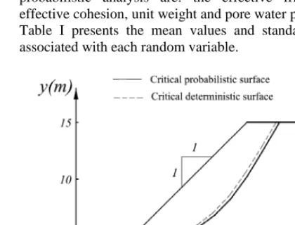
Figure 4 shows the geometry of a slope in homogeneous soil. The parameters considered as random variables in the probabilistic analysis are: the effective friction angle, effective cohesion, unit weight and pore water pressure ratio. Table I presents the mean values and standard deviation associated with each random variable.

TABLEI

STATISTICAL PROPERTIES OF SOIL PARAMETERS- EXAMPLE 1

Random variable

Mean Standard deviation

Distribution

c' 18.0kN/m2 3.6kN/m2 Log-normal

tan φ' tan 30 0.0577 Log-normal

γ 18.0kN/m3 _0.9kN/m3 _Log-normal

ru 0.2 0.02 Log-normal

The problem was previously solved by Li and Lumb [10], Hassan and Wolff [1] and Bhattacharya et al. [2]. The results of the proposed method and previous studies are summarized in Table II.

In Table II, FSmin and βFS are the minimum factor of safety

and the reliability index associated with the critical

deterministic slip surface, respectively, and βmin is the

minimum reliability index corresponding to the critical probabilistic slip surface.

According to analysing the results of this table, it can be observed that, the minimum reliability index calculated using presented method is 2.212, which is lower than the values reported by Li and Lumb (2.5) Hassan and Wolff (2.293), Bhattacharya et al. (2.239). Further, the minimum factor of safety calculated from a deterministic analysis based on the mean values of the soil properties obtained by PSO is 1.309, which is lower than 1.326 reported by Bhattacharya et al. [2].

The corresponding critical deterministic and the critical probabilistic slip surfaces are also presented in Fig. 4. As it can be seen, two surfaces are located reasonably close to each other as expected in a homogeneous slope. It’s because

of the proximity of the values of βFS and βmin presented in

Table II. The failure surfaces reported by previous researchers are also similarly located.

TABLEII

RESULTS COMPARISON- EXAMPLE 1

Method βFS βmin FSmin

Li and Lumb [10] - 2.5 -

Hassan and Wolff [1] 2.336 2.293 -

Bhattacharya et al [2] 2.306 2.239 1.326

Present study (PSO) 2.295 2.212 1.309

B. Example 2

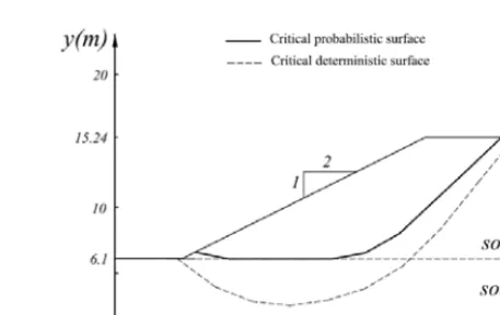
Figure 5 shows the cross section and geometry of a two layered slope in clay bounded by a hard layer below and parallel to the ground surface. The soil strength parameters that are related to the stability of slope, including friction

angle φ, and cohesion c, are considered as random variables.

The statistical moments (mean value and standard deviation) of the parameters are summarized in Table III.

This example was also solved previously by Hassan and

Wolff [1] and Bhattacharya et al [2] in terms of FSmin, βFS

and βmin. The results obtained from current study together with a comparison of those reported by previous researchers are summarized in Table IV. For the results shown in this table, it can be considered that the minimum reliability index evaluated using PSO is 2.771, which is almost lower than those reported by Hassan and Wolff [1] and Bhattacharya et

al. [2]. Besides, the minimum factor of safety obtained by PSO is found to be smaller than the others. The corresponding critical deterministic and the critical probabilistic slip surfaces are presented in Fig. 5. In

accordance with the difference in the values of βFS and βmin

presented in Table IV, the two surfaces are located significantly separate.

Fig. 5 Cross section of non homogeneous slope-example 2

TABLEIII

STATISTICAL PROPERTIES OF SOIL PARAMETERS- EXAMPLE 2

Material Parameter Mean Standard

deviation

Distribution

Soil 1 c1 38.31kN/m2 7.662kN/m2 Log-normal

φ1 0 - Log-normal

Soil 2 c2 23.94kN/m2 4.788kN/m2 Log-normal

φ2 12 1.2 Log-normal

TABLEIV

RESULTS COMPARISON- EXAMPLE 2

Method βFS βmin FSmin

Hassan and Wolff [1] 4.442 2.869 1.663

Bhattacharya et al [2] 5.064 2.861 1.665

Present study (PSO) 4.545 2.771 1.655

V. CONCLUSIONS

This paper outlines a procedure of probabilistic analysis

of earth slope. The Hasofer-Lind reliability index (βHL) is

used instead of the conventional reliability index β. The

problem of searching the critical probabilistic surface with

the minimum reliability index, βmin, can be formulated as an

surface is almost close for slope in a homogenous soil whereas these surfaces are located quite separate for non homogenous slopes.

REFERENCES

[1] A. Hassan, and T. Wolff, “Search algorithm for minimum reliability

index of earth slopes,” J. Geotech. Goenviron. Vol. 125, pp.

301-308, 1999.

[2] G. Bhattacharya, D. Jana, S. Ojha and S. Chakraborty, “Direct

search for minimum reliability index of earth slopes,” Comput.

Geotech. Vol. 30, No. 6, pp. 455-462, 2003.

[3] D. Tobutt, and E. Richards, “The reliability of earth slopes,” Int. J.

Numer.Anal. met. Vol. 3 No. 4, pp. 323-354, 2005.

[4] S. Cho, “Effects of spatial variability of soil properties on slope

stability,” Eng. Geol. Vol. 92 No. 3-4, pp. 97-109, 2007.

[5] G. Xie, J. Zhang, and J. Li, “Adapted Genetic Algorithm Applied to

Slope Reliability Analysis,” Fourth International Conference on

Natural Computation, pp. 520-524, 2008.

[6] A. Hasofer, and N. Lind, “Exact and invariant second-moment code

format,” J. Eng. Mech-ASCE. Vol. 100, No. 1, pp. 111-121,

1974.

[7] J. Kennedy, and R. Eberhart, “Particle swarm optimization,” In

Proc.IEEE International Conference on Neural Networks, 1995, pp. 1942-1948

[8] A. W. Bishop, “The use of the slip circle in the stability analysis of

earth slopes,”.Geotechinque, vol. 5, No. 1, pp. 7-17, 1955.

[9] Y. Shi, and R. Eberhart, “A modified particle swarm optimizer,” In

Proc.IEEE World Congress on Evolutionary Computation, 1998, p. 69-73.

[10] K. Li, and P. Lumb, “Probabilistic design of slopes,” Can. Geotech.