National Semiconductor’
s
CONTENTS
1. Introduction to this Handbook ... 1
2. Temperature Sensing Techniques... 1
RTDs
... 1
Thermistors
... 2
Thermocouples
... 3
Silicon Temperature Sensors
... 4
3 National’s Temperature Sensor ICs ...5
3.1 Voltage-Output Analog Temperature Sensors
... 5
LM135, LM235, LM335 Kelvin Sensors
... 5
LM35, LM45 Celsius Sensors
... 5
LM34 Fahrenheit Sensor
... 6
LM50 “Single Supply” Celsius Sensor
... 6
LM60 2.7V Single Supply Celsius Sensor
... 6
3.2 Current-Output Analog Sensors
... 6
LM134, LM234, and LM334 Current-Output Temperature Sensors
... 6
3.3 Comparator-Output Temperature Sensors
... 7
LM56 Low-Power Thermostat
... 7
3.4 Digital Output Sensors
... 8
LM75 Digital Temperature Sensor and Thermal Watchdog With Two-Wire Interface
... 8
LM78 System Monitor
... 9
4. Application Hints... 10
Sensor Location for Accurate Measurements
... 10
Example 1. Audio Power Amplifier
... 11
Example 2. Personal Computer
... 12
Example 3. Measuring Air Temperature
... 13
Mapping Temperature to Output Voltage or Current
... 13
Driving Capacitive Loads (These hints apply to analog-output sensors)
... 14
Noise Filtering
... 14
5. Application Circuits ...15
5.1 Personal Computers
... 15
Simple Fan Controller
... 15
Low/High Fan Controllers
... 16
Digital I/O Temperature Monitor
... 17
5.2 Interfacing External Temperature Sensors to PCS
... 18
5.4 Audio
... 22
Audio Power Amplifier Heat Sink Temperature Detector and Fan Controller
... 22
5.5 Other Applications
... 23
Two-Wire Temperature Sensor
... 23
4-to-20mA Current Transmitter (0°C to 100°C)
... 24
Multi-Channel Temperature-to-Digital Converter
... 25
Oven Temperature Controllers
... 25
Isolated Temperature-to-Frequency Converter
... 26
6. Datasheets... 27
LM34
... 29
LM35
... 30
LM46
... 31
LM50
... 32
LM56
... 33
LM60
... 34
LM75
... 35
LM77
... 36
LM78
... 37
LM80
... 38
LM134
... 39
1. Introduction to This Handbook
Temperature is the most often-measured environmental quantity. This might be expected since most physical, electronic, chemical, mechanical and biological systems are affected by temperature. Some processes work well only within a narrow range of temperatures; certain chemical reactions, biological processes, and even electronic circuits perform best within limited temperature ranges. When these processes need to be optimized, control sys-tems that keep temperature within specified limits are often used. Temperature sensors provide inputs to those control systems.
Many electronic components can be damaged by exposure to high temperatures, and some can be damaged by exposure to low temperatures. Semiconductor devices and LCDs (Liquid Crystal Displays) are examples of com-monly-used components that can be damage by temperature extremes. When temperature limits are exceeded, action must be taken to protect the system. In these systems, temperature sensing helps enhance reliability. One example of such a system is a personal computer. The computer’s motherboard and hard disk drive gener-ate a great deal of heat. The internal fan helps cool the system, but if the fan fails, or if airflow is blocked, sys-tem components could be permanently damaged. By sensing the sys-temperature inside the computer’s case, high-temperature conditions can be detected and actions can be taken to reduce system high-temperature, or even shut the system down to avert catastrophe.
Other applications simply require temperature data so that temperatures effect on a process may be accounted for. Examples are battery chargers (batteries’ charge capacities vary with temperature and cell temperature can help determine the optimum point at which to terminate fast charging), crystal oscillators (oscillation frequen-cy varies with temperature) and LCDs (contrast is temperature-dependent and can be compensated if the tem-perature is known).
This handbook provides an introduction to temperature sensing, with a focus on silicon-based sensors. Included are several example application circuits, reprints of magazine articles on temperature sensing, and a selection guide to help you choose a silicon-based sensor that is appropriate for your application.
2. Temperature Sensing Techniques
Several temperature sensing techniques are currently in widespread usage. The most common of these are RTDs, thermocouples, thermistors, and sensor ICs. The right one for your application depends on the required temperature range, linearity, accuracy, cost, features, and ease of designing the necessary support circuitry. In this section we discuss the characteristics of the most common temperature sensing techniques.
RTDs
Resistive sensors use a sensing element whose resistance varies with temperature. A platinum RTD
(Resistance Temperature Detector) consists of a coil of platinum wire wound around a bobbin, or a film of plat-inum deposited on a substrate. In either case, the sensors resistance-temperature curve is a nearly-linear func-tion, as shown in Figure 2.1. The RTDs resistance curve is the lower one; a straight line is also shown for refer-ence. Nonlinearity is several degrees at temperature extremes, but is highly predictable and repeatable. Correction of this nonlinearity may be done with a linearizing circuit or by digitizing the measured resistance value and using a lookup table to apply correction factors. Because of the curve’s high degree of repeatability over a wide temperature range (roughly -250 degrees C to +750 degrees C), and platinums stability (even when hot), you’ll find RTDs in a variety of precision sensing applications.
300 400 500
RTD Resistance vs Temperature
Complexity of RTD signal processing circuitry varies substantially depending on the application. Usually, a known, accurate current is forced through the sensor, and the voltage across the sensor is measured. Several components, each of which generates its own errors, are necessary. When leads to the sensor are long, four-wire connections to the sensor can eliminate the effects of lead resistance, but this may increase the amplifier’s complexity.
Low-voltage operation is possible with resistive sensors — there are no inherent minimum voltage limitations on these devices — and there are enough precision low-voltage amplifiers available to make low voltage operation reasonable to achieve. Low-power operation is a little tougher, but it can be done at the expense of complexity by using intermittent power techniques. By energizing the sensor only when a measurement needs to be made, power consumption can be minimized.
RTDs have drawbacks in some applications. For example, the cost of a wire-wound platinum RTD tends to be relatively high. On the other hand, thin-film RTDs and sensors made from other metals can cost as little as a few dollars. Also, self-heating can occur in these devices. The power required to energize the sensor raises its temperature, which affects measurement accuracy. Circuits that drive the sensor with a few mA of current can develop self-heating errors of several degrees. The non-linearity of the resistance-vs.-temperature curve is a disadvantage in some applications, but as mentioned above, it is very predictable and therefore correctable.
Thermistors
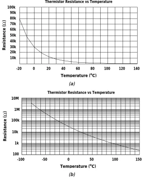
Another type of resistive sensor is the thermistor. Low-cost thermistors often perform simple measurement or trip-point detection functions in low-cost systems. Low-precision thermistors are very inexpensive; at higher price points, they can be selected for better precision at a single temperature. A thermistors resistance-temperature function is very nonlinear (Figure 2.2), so if you want to measure a wide range of temperatures, you’ll find it necessary to perform substantial linearization. An alternative is to purchase linearized devices, which generally consist of an array of two thermistors with some fixed resistors. These are much more expensive and less sensitive than single thermistors, but their accuracy can be excellent.
Simple thermistor-based set-point thermostat or controller applications can be implemented with very few components - just the thermistor, a comparator, and a few resistors will do the job.
(a)
[image:5.612.158.452.334.700.2](b)
Figure 2.2. Thermistor Resistance vs. Temperature. (a) linear scale. (b) logarithmic scale.
150 100
50 0
-50 -100
Thermistor Resistance vs Temperature
Temperature (oC)
10M 1M 100k 10k
1k 100
Resistance (
)
140 120 100 80 60 40 20 0 -20
Thermistor Resistance vs Temperature
Temperature (oC)
10k 100k
20k 30k 40k 50k 60k 70k 80k 90k
Resistance (
When functionality requirements are more involved (for example if multiple trip points or analog-to-digital conversion are necessary), external circuitry and cost increase quickly. Consequently, you’ll typically use low-cost thermistors only in applications with minimal functionality requirements. Thermistors can be affected by self-heating, usually at higher temperatures where their resistances are lower. As with RTDs, there are no fun-damental reasons why thermistors shouldn’t be used on low supply voltages. External active components such as comparators or amplifiers will usually limit the low end of the supply voltage range. You can find thermis-tors that will work over a temperature range from about -100°C to +550°C although most are rated for maxi-mum operating temperatures from 100°C to 150°C.
Thermocouples
A thermocouple consists of a junction of two wires made of different materials. For example, a Type J thermo-couple is made from iron and constantan wires, as shown in Figure 2.3. Junction 1 is at the temperature to be measured. Junctions 2 and 3 are kept at a different, known temperature. The output voltage is approximately proportional to the difference in temperature between Junction 1 and Junctions 2 and 3. Typically, you’ll mea-sure the temperature of Junctions 2 and 3 with a second sensor, as shown in the figure. This second sensor enables you to develop an output voltage proportional to an appropriate scale (for example, degrees C), by adding a voltage to the thermocouple output that has the same slope as that of the thermocouple, but is relat-ed to the temperature of the junctions 2 and 3.
Figure 2.3.
Because a thermocouples “sensitivity” (as reflected in its Seebeck coefficient) is rather small — on the order of tens of microvolts per degree C — you need a low-offset amplifier to produce a usable output voltage.
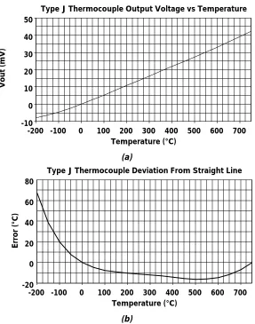
Nonlinearities in the temperature-to-voltage transfer function (shown in Figure 2.4) amount to many degrees over a thermocouples operating range and, as with RTDs and thermocouples, often necessitate compensation circuits or lookup tables. In spite of these drawbacks, however, thermocouples are very popular, in part because of their low thermal mass and wide operating temperature range, which can extend to about 1700°C with com-mon types. Table 2.1 shows Seebeck coefficients and temperature ranges for a few thermocouple types.
R2 505 R1
100k LM35
Cold-junction compensated output. 50.2 V/oC +5V
Thermocouple Measurement Junction
Copper
Copper Iron
Constantan
10mV/oC 1
2
(a)
(b)
[image:7.612.163.450.45.410.2]Figure 2.4. (a) Output voltage as a function of temperature for a Type J thermocouple. b) Approximate error in °C vs. a straight line that passes through the curve at 0°C and 750°C
Table 2.1. Seebeck Coefficients and Temperature Ranges for various thermocouple types.
Silicon Temperature Sensors
Integrated circuit temperature sensors differ significantly from the other types in a couple of important ways. The first is operating temperature range. A temperature sensor IC can operate over the nominal IC temperature range of -55°C to +150°C. Some devices go beyond this range, while others, because of package or cost con-straints, operate over a narrower range. The second major difference is functionality. A silicon temperature sensor is an integrated circuit, and can therefore include extensive signal processing circuitry within the same package as the sensor. You don’t need to design cold-junction compensation or linearization circuits for tem-perature sensor ICs, and unless you have extremely specialized system requirements, there is no need to design comparator or ADC circuits to convert their analog outputs to logic levels or digital codes. Those func-tions are already built into several commercial ICs.
Type Seebeck Coefficient Temperature Range
µV/°C (°C)
E 58.5@0°C 0 to 1700
J 50.2@0°C 0 to 750
K 39.4@0°C -200 to 1250
R 11.5@0°C 0 to 1450
700 600 500 400 300 200 100 0 -100 -200 -200 -20
0 20 40 60 80
Type J Thermocouple Deviation From Straight Line
Temperature (°C)
Error (°C)
700 600 500 400 300 200 100 0 -100 -200 -200 -10
0 10 20 30 40 50
Type J Thermocouple Output Voltage vs Temperature
Temperature (°C)
3. National’s Temperature Sensor ICs
National builds a wide variety of temperature sensor ICs that are intended to simplify the broadest possible range of temperature sensing challenges. Some of these are analog circuits, with either voltage or current out-put. Others combine analog sensing circuits with voltage comparators to provide “thermostat” or “alarm” func-tions. Still other sensor ICs combine analog sensing circuitry with digital I/O and control registers, making them an ideal solution for microprocessor-based systems such as personal computers.
Below is a summary of National’s sensor products as of August, 1996. Unless otherwise noted, the specifica-tions listed in this section are the guaranteed limits for the best grade device.
3.1 Voltage-Output Analog Temperature Sensors
LM135, LM235, LM335 Kelvin Sensors
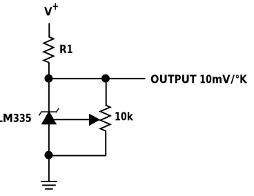
[image:8.612.215.399.288.430.2]The LM135, LM235, and LM335 develop an output voltage proportional to absolute temperature with a nomi-nal temperature coefficient of 10mV/K. The nominomi-nal output voltage is therefore 2.73V at 0°C, and 3.73V at 100°C. The sensors in this family operate like 2-terminal shunt voltage references, and are nominally connect-ed as shown in Figure 3.1. The third terminal allows you to adjust accuracy using a trimpot as shown in the Figure. The error of an untrimmed LM135A over the full -55°C to +150°C range is less than ±2.7°C. Using an external trimpot to adjust accuracy reduces error to less than ±1°C over the same temperature range. The sen-sors in this family are available in the plastic TO-92 and SO-8 packages, and in the TO-46 metal can.
Figure 3.1. Typical Connection for LM135, LM235, and LM335. Adjust the potentiometer for the correct output voltage at a known temperature (for example 2.982V @ 25°C), to obtain better than ±1°C accuracy over the -55°C to +150°C temperature range.
LM35, LM45 Celsius Sensors
The LM35 and LM45 are three-terminal devices that produce output voltages proportional to °C (10mV/°C), so the nominal output voltage is 250mV at 25°C and 1.000V at 100°C. These sensors can measure temperatures below 0°C by using a pull-down resistor from the output pin to a voltage below the “ground” pin (see the “Applications Hints” section). The LM35 is more accurate (±1°C from -55°C to +150°C vs. ±3°C from -20°C to +100°C), while the LM45 is available in the “Tiny” SOT-23 package. The LM35 is available in the plastic TO-92 and SO-8 packages, and in the TO-46 metal can.
LM35 +Vs
(+5V to +20V)
OUTPUT
VOUT= +10mV/°F
OUTPUT
VOUT= +10mV/°C +Vs
(+5V to +20V)
OUTPUT
VOUT= +10mV/°C +Vs
(+4V to +10V)
LM45 LM34
V+
R1
OUTPUT 10mV/°K
LM34 Fahrenheit Sensor
The LM34 is similar to the LM35, but its output voltage is proportional to °F (10mV/°F). Its accuracy is similar to the LM35 (±2°F from -50°F to +300°F), and it is available in the same TO-92, SO-8, and TO-46 packages as the LM35.
LM50 “Single Supply” Celsius Sensor
The LM50 is called a “Single Supply” Celsius Sensor because, unlike the LM35 and LM45, it can measure nega-tive temperatures without taking its output pin below its ground pin (see the “Applications Hints” section). This can simplify external circuitry in some applications. The LM50’s output voltage has a 10mV/°C slope, and a 500mV “offset”. Thus, the output voltage is 500mV at 0°C, 100mV at -40°C, and 1.5V at +100°C. Accuracy is with-in 3°C over the full -40°C to +125°C operatwith-ing temperature range. The LM50 is available with-in the SOT-23 package.
Figure 3.3. LM50 Typical Connection
LM60 2.7V Single Supply Celsius Sensor
The LM60 is similar to the LM50, but is intended for use in applications with supply voltages as low as 2.7V. Its 110µA supply current drain is low enough to make the LM60 an ideal sensor for battery-powered systems. The LM60’s output voltage has a 6.25mV/°C slope, and a 424mV “offset”. This results in output voltages of 424mV at 0°C, 174mV at -40°C, and 1.049V at 100°C. The LM60 is available in the SOT-23 package.
Figure 3.4. LM60 Typical Connection
3.2 Current-Output Analog Sensors
LM134, LM234, and LM334 Current-Output Temperature Sensors
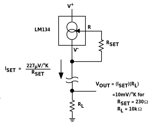
Although its data sheet calls it an “adjustable current source”, the LM134 is also a current-output temperature sensor with an output current proportional to absolute temperature. The sensitivity is set using a single exter-nal resistor. Typical sensitivities are in the 1µA/°C to 3µA/°C range, with 1µA/°C being a good nomiexter-nal value. By adjusting the value of the external resistor, the sensitivity can be trimmed for good accuracy over the full oper-ating temperature range (-55°C to +125°C for the LM134, -25°C to +100°C for the LM234, and 0°C to +70°C for the LM334). The LM134 typically needs only 1.2V supply voltage, so it can be useful in applications with very limited voltage headroom. Devices in this family are available in SO-8 and TO-92 plastic packages and TO-46 metal cans.
LM60 OUTPUT
VOUT= 6.25mV/°C + 424mV V+
(2.7V to 10V)
LM50 OUTPUT
VOUT= 10mV/°C + 500mV V+
Figure 3.5. LM134 Typical Connection. RSETcontrols the ratio of output current to temperature.
3.3 Comparator-Output Temperature Sensors
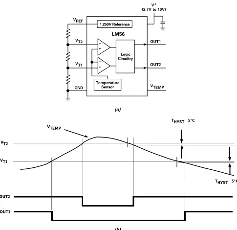
LM56 Low-Power Thermostat
The LM56 includes a temperature sensor (similar to the LM60), a 1.25V voltage reference, and two compara-tors with preset hysteresis. It will operate from power supply voltages between 2.7V and 10V, and draws a maximum of 200µA from the power supply. The operating temperature range is -40°C to +125°C. Comparator trip point tolerance, including all sensor, reference, and comparator errors (but not including external resistor errors) is 2°C from 25°C to 85°C, and 3°C from -40°C to +125°C.
The internal temperature sensor develops an output voltage of 6.2mV x T(°C) + 395mV. Three external resistors set the thresholds for the two comparators.
V+
LM134
V-R
RSET
RL
VOUT = (ISET)(RL) =10mV/oK for
RSET = 230 RL = 10k ISET = 227 V/
oK
(a)
[image:11.612.65.550.50.520.2](b)
Figure 3.6. (a) LM56 block diagram. (b) Comparator outputs as a function of temperature.
3.4 Digital Output Sensors
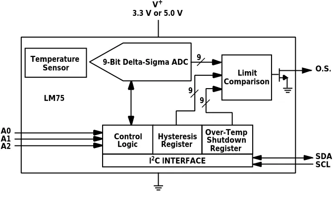
LM75 Digital Temperature Sensor and Thermal Watchdog With Two-Wire Interface
The LM75 contains a temperature sensor, a delta-sigma analog-to-digital converter (ADC), a two-wire digital interface, and registers for controlling the IC’s operation. The two-wire interface follows the I2C®protocol.
Temperature is continuously being measured, and can be read at any time. If desired, the host processor can instruct the LM75 to monitor temperature and take an output pin high or low (the sign is programmable) if temperature exceeds a programmed limit. A second, lower threshold temperature can also be programmed, and the host can be notified when temperature has dropped below this threshold. Thus, the LM75 is the heart of a temperature monitoring and control subsystem for microprocessor-based systems such as personal com-puters. Temperature data is represented by a 9-bit word (1 sign bit and 8 magnitude bits), resulting in 0.5°C resolution. Accuracy is ±2°C from -25°C to +100°C and ±3°C from -55°C to +125°C. The LM75 is available in an 8-pin SO package.
OUT1 OUT2 VT1 VT2
VTEMP
THYST 5°C THYST 5°C
I2
Figure 3.7. LM75 Block Diagram.
LM78 System Monitor
The LM78 is a highly-integrated Data Acquisition system IC that can monitor several kinds of analog inputs simultaneously, including temperature, frequency, and analog voltage. It is an ideal single-chip solution for improving the reliability of servers, Personal Computers, or virtually any microprocessor-based instrument or system. The IC includes a temperature sensor, I2C and ISA interfaces, a multiple-input 8-bit ADC (five positive inputs and 2 negative inputs), fan speed counters, several control and memory registers, and numerous other functions. In a PC, the LM78 can be used to monitor power supply voltages, temperatures, and fan speeds. The values of these analog quantities are continuously digitized and can be read at any time. Programmable
WATCHDOG™ limits for any of these analog quantities activate a fully-programmable and maskable interrupt system with two outputs. An input is provided for the overtemperature outputs of additional temperature sen-sors (such as the LM56 and LM75) and this is linked to the interrupt system. Additional inputs are provided for Chassis Intrusion detection circuits, VID monitor inputs, and chainable interrupt. A 32-byte auto-increment RAM is provided for POST (Power On Self Test) code storage.
The LM78 operates from a single 5V power supply and draws less than 1mA of supply current while operating. In shutdown mode, supply current drops to 10µA.
Temperature Sensor
Limit Comparison
Control Logic
Over-Temp Shutdown Register
I2C INTERFACE SDA
SCL O.S.
A0 A1 A2
V+ 3.3 V or 5.0 V
9
Hysteresis Register LM75
9-Bit Delta-Sigma ADC
Figure 3.8. The LM78 is a highly-integrated system monitoring circuit that tracks not only temperature, but also power supply voltages, fan speed, and other analog quantities.
4. Application Hints
The following Application Hints apply to most of National’s temperature sensor ICs. For hints that are specific to a particular sensor, please refer to that sensors data sheet.
Sensor Location for Accurate Measurements
A temperature sensor produces an output, whether analog or digital, that depends on the temperature of the sensor. Heat is conducted to the sensing element through the sensors package and its metal leads. In general, a sensor in a metal package (such as an LM35 in a TO46) will have a dominant thermal path through the pack-age. For sensors in plastic packages like TO-92, SO-8, and SOT-23, the leads provide the dominant thermal path. Therefore, a board-mounted IC sensor will do a fine job of measuring the temperature of the circuit board (especially the traces to which the leads are soldered). If the board’s temperature is very close to the ambient air temperature (that is, if the board has no significant heat generators mounted on it), the sensors temperature will also be very near that of the ambient air.
If you want to measure the temperature of something other than the circuit board, you must ensure that the sensor and its leads are at the same temperature as the object you wish to measure. This usually involves mak-ing a good mechanical and thermal contact by, for example, attachmak-ing the sensor (and its leads) to the object being measured with thermally-conductive epoxy. If electrical connections can be made directly from the sen-sors leads to the object being measured, soldering the leads of an IC sensor to the object will give a good ther-mal connection. If the ambient air temperature is the same as that of the surface being measured, the sensor will be within a fraction of a degree of the surface temperature. If the air temperature is much higher or lower
Limit Registers and WATCHDOG Comparators LM75 Digital Temperature Sensor +5V Chassis Intrusion Detector Chassis Intrusion Fan Inputs Positive Analog Inputs +12V Interrupt Masking and Interrupt Control
Interface and Control Fan Speed Counter — + — + Temperature Sensor Negative Analog Inputs 8-Bit ADC Interrupt Outputs ISA Interface S D A S C L +5V
To power supply voltages, analog temperature sensors,
than the surface temperature, the temperature of the sensor die will be at an inter-mediate temperature
between the surface temperature and the air temperature. A sensor in a plastic package (a TO-92 or SOT-23, for example) will indicate a temperature very close to that of its leads (which will be very close to the circuit board’s temperature), with air temperature having a less significant effect. A sensor in a metal package (like a TO-46) will usually be influenced more by air temperature. The influence of air temperature can be further increased by gluing or clamping a heat sink to the metal package.
If liquid temperature is to be measured, a sensor can be mounted inside a sealed-end metal tube, and can then be dipped into a bath or screwed into a threaded hole in a tank. Temperature sensors and any accompanying wiring and circuits must be kept insulated and dry, to avoid leakage and corrosion. This is especially true for IC temperature sensors if the circuit may operate at cold temperatures where condensation can occur. Printed-cir-cuit coatings and varnishes such as Humiseal and epoxy paints or dips are often used to ensure that moisture cannot corrode the sensor or its connections.
So where should you put the sensor in your application? Here are three examples:
Example 1. Audio Power Amplifier
It is often desirable to measure temperature in an audio power amplifier to protect the electronics from over-heating, either by activating a cooling fan or shutting the system down. Even an IC amplifier that contains internal circuitry to shut the amplifier down in the event of overheating (National’s Overture™-series ampli-fiers, for example) can benefit from additional temperature sensing. By activating a cooling fan when tempera-ture gets high, the system can produce more output power for longer periods of time, but still avoids having the fan (and producing noise) when output levels are low.
Audio amplifiers that dissipate more than a few watts virtually always have their power devices (either discrete transistors or an entire monolithic amplifier) bolted to a heat sink. The heat sinks temperature depends on ambient temperature, the power device’s case temperature, the power device’s power dissipation, and the thermal resistance from the case to the heat sink. Similarly, the power device’s case temperature depends on the device’s power dissipation and the thermal resistance from the silicon to the case. The heat sinks tempera-ture is therefore not equal to the “junction temperatempera-ture”, but it is dependent on it and related to it.
A practical way to monitor the power device’s temperature is to mount the sensor on the heat sink. The sen-sors temperature will be lower than that of the power device’s die, but if you understand the correlation between heat sink temperature and die temperature, the sensors output will still be useful.
Figure 4.1 shows an example of a monolithic power amplifier bolted to a heat sink. Next to the amplifier is a temperature sensor IC in a TO-46 metal can package. The sensor package is in a hole drilled into the heat sink; the sensor is cemented to the heat sink with heat-conducting epoxy. Heat is conducted from the heat sink through the sensors case, and from the circuit board through the sensors leads. Depending on the amplifier, the heat sink, the printed circuit board layout, and the sensor, the best indication of the amplifier’s temperature may be obtained through the metal package or through the sensors leads.
The amplifier IC’s leads will normally be within a few degrees of the temperature of the heat sink near the amplifier. If the amplifier is soldered directly to the printed circuit board, and if the leads are short, the circuit board traces at the amplifier’s leads will be quite close to the heat sink temperature — sometimes higher, sometimes lower, depending on the thermal characteristics of the system. Therefore, if the sensor can be sol-dered to a point very close to the amplifier’s leads, you’ll get a good correlation with heat sink temperature. This is especially good news if you’re using a temperature sensor in a plastic package, since thermal conduc-tion for such a device is through the leads. Locate the sensor as close as possible to the amplifier’s leads. If the amplifier has a ground pin, place the sensors ground pin right next to that of the amplifier and try to keep the other sensor leads at the same temperature as the amplifier’s leads.
Figure 4.1. TO-220 power amplifier and TO-46 sensor mounted on heat sink. Excellent results can also be obtained by locating the sensor on the circuit board very close to the amplifier IC’s leads.
Example 2. Personal Computer
High-performance microprocessors such as the Pentium®or Power PC®families consume a lot of power and
can get hot enough to suffer catastrophic damage due to excessive temperature. To enhance system reliability, it is often desirable to monitor processor temperature and activate a cooling fan, slow down the system clock, or shut the system down completely if the processor gets too hot.
As with power amplifiers, there are several potential mounting sites for the sensor. One such location is in the center of a hole drilled into the microprocessors heat sink, shown as location “a” in Figure 4.2. The heat sink, which can be clipped to the processor or attached with epoxy, generally sits on top of the processor. The advantage of this location is that the sensors temperature will be within a few degrees of the microprocessors case temperature in a typical assembly. A disadvantage is that relatively long leads will be required to return the processor’s output to the circuit board. Another disadvantage is that if the heat-sink-to-microprocessor thermal connection degrades (either because of bad epoxy or because a clip-on heat sink gets “bumped” and is no longer in intimate contact with the processor), the sensor-to-microprocessor connection will probably also be disrupted, which means that the sensor will be at a lower than normal temperature while the processor temperature is rising to a potentially damaging level.
Another potential location is in the cavity beneath a socketed processor (Figure 4.2, location “b”). An advan-tage of this site is that, since the sensor is attached to the circuit board using conventional surface-mounting techniques, assembly is straightforward. Another advantage is that the sensor is isolated from air flow and will not be influenced excessively by changes in ambient temperature, fan speed, or direction of cooling air flow. Also, if the heat sink becomes detached from the microprocessor, the sensor will indicate an increase in micro-processor temperature. A disadvantage is that the thermal contact between the sensor and the micro-processor is not as good as in the previous example, which can result in temperature differences between the sensor and the microprocessor case of 5°C to 10°C. This is only a minor disadvantage, however, and this approach is the most practical one in many systems.
It is also possible to mount the sensor on the circuit board next to the microprocessors socket (location “c”). This is another technique that is compatible with large-volume manufacturing, but the correlation between sensor temperature and processor temperature is much weaker (the microprocessor case can be as much as 20°C warmer than the sensor).
Figure 4.2. Three potential sensor locations for high-performance processor monitoring.
Hole drilled in heatsink
Pentium or Similar Processor
PCB b a
c Socket
Finally, in some lower-cost systems the microprocessor may be soldered to the motherboard, with the heat sink mounted on the opposite side of the motherboard, as shown in Figure 4.3. In these systems, the sensor can be soldered to the board at the edge of the heat sink. Since the microprocessor is in close contact with the mother-board, the sensors temperature will be closer to that of the microprocessor than for a socketed microprocessor.
Figure 4.3. Sensor mounted near edge of soldered processor.
Example 3. Measuring Air Temperature
Because the sensors leads are often the dominant thermal path, a board-mounted sensor will usually do an excellent job of measuring board temperature. But what if you want to measure air temperature? If the board is at the same temperature as the air, you’re in luck.
If the board and the air are at different temperatures, things get more complicated. The sensor can be isolated from the board using long leads. If the sensor is in a metal can, a clip-on heat sink can bring the sensors tem-perature close to ambient. If the sensor is in a plastic package, it may need to be mounted on a small “sub-board”, which can then be thermally isolated from the main board with long leads.
For more information on finding the ideal location for a temperature sensor, refer to the article “Get Maximum Accuracy From Temperature Sensors” by Jerry Steele (Electronic Design, August 19, 1996).
Mapping Temperature to Output Voltage or Current
The earliest analog-output temperature sensors developed by National generated output signals that were pro-portional to absolute temperature (K). The LM135 series has a nominal output voltage equal to 10mV/K, while the LM134 series (a current-output device) produces a current proportional to absolute temperature. The scal-ing factor is determined by an external resistor.
Because the Celsius and Fahrenheit scales are more convenient in many applications, three of our sensors have output voltages proportional to one of those scales. The LM35 and LM45 produce nominal output volt-ages equal to 10mV/°C, while the LM34 produces a nominal output equal to 10mV/°F.
While the Celsius and Fahrenheit sensors have more convenient temperature-to-voltage mapping than the absolute temperature sensors, they are somewhat less convenient to use when you need to look at tempera-tures below 0°C or 0°F. To measure “negative” temperatempera-tures with these devices, you need to either provide a negative power supply as in Figure 4.4(a), or bias the sensor above ground and look at the voltage differential between its output and “ground” pins as in Figure 4.4(b).
R1 VOUT
V-LM45
V+
(4V to 10V) Choose R1 = -V-/50µA
VOUT = 10mV/°C = 1.00V @ 100°C = 250mV @ 25°C = 0V @ 0°C = -200mV @ -20°C
R1 VOUT LM45
V+ (4V to 10V)
VOUT PCB
Ground Plane Feedthroughs Pentium or Similar Processor
The LM50 and LM60 use an alternative approach. These devices have a built-in positive offset voltage that allows them to produce output voltages corresponding to negative temperatures when operating on a single positive supply. The LM50 has a 10mV/°C scale factor, but the output voltage is 500mV at 0°C. The device is specified for temperatures as low as -40°C (100mV). The LM60’s scale factor is 6.25mV/°C, and its output volt-age is 424mV at 0°C. The LM60 also is specified for temperatures as low as -40°C (174mV).
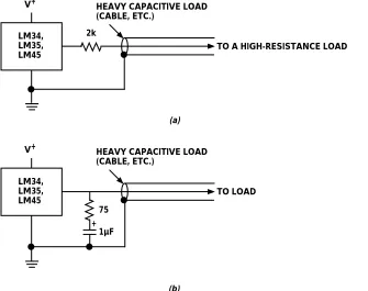
Driving Capacitive Loads (These hints apply to analog-output sensors).
[image:17.612.144.479.214.479.2]National’s temperature sensor ICs are micropower circuits, and like most micropower circuits, they generally have a limited ability to drive heavy capacitive loads. The LM34 and LM35, for example, can drive 50pF without special precautions, while the LM45 can handle 500pF. If heavier capacitive loads are anticipated, it is easy to isolate or decouple the load with a resistor; see Figure 4.5. Note that the series resistor will attenuate the out-put signal unless the load resistance is very high. If this is a problem, you can improve the tolerance to capaci-tive loading without increasing output resistance by using a series R-C damper from output to ground as shown in Figure 4.5.
Figure 4.5. Capacitive drive options. The LM34, LM35, and LM45 can drive large external capacitance if isolated from the load capacitance with a resistor as in (a), or compensated with an R-C network as in (b).
The LM50 and LM60 have internal isolation resistances and can drive any value of capacitance with no stability problems. Ensure that the load impedance is sufficiently high to avoid attenuation of the output signal,
Noise Filtering
Any linear circuit connected to wires in a hostile environment can have its performance adversely affected by intense electromagnetic sources such as relays, radio transmitters, motors with arcing brushes, SCR transients, etc., as its wiring can act as a receiving antenna and its internal junctions can act as rectifiers. In such cases, a 0.1µF bypass capacitor from the power supply pin to ground will help clean up power supply noise. Output fil-tering can be added as well. Sensors like the LM50 and LM60 can drive filter capacitors directly; a 1µF to 4.7µF output capacitor generally works well. When using sensors that should not directly drive large capacitive loads, you can isolate the filter capacitor with a resistor as shown in Figure 4.5(a), or use the R-C damper in Figure 4.5(b) to provide filtering. Typical damper component values are 75Ωin series with 0.2µF to 1µF.
V+
2k LM34,
LM35, LM45
TO A HIGH-RESISTANCE LOAD HEAVY CAPACITIVE LOAD
(CABLE, ETC.)
(a)
(b) V+
75
1µF + LM34,
LM35, LM45
TO LOAD HEAVY CAPACITIVE LOAD
5. Application Circuits
5.1 Personal Computers
Recent generations of personal computers dissipate a lot of power, which means they tend to run hot. The microprocessor and the hard disk drive are notable hot spots. Cooling fans help to keep heat under control, but if a fan fails, or if ventilation paths become blocked by dust or desk clutter, the temperature inside a com-puter’s case can get high enough to dramatically reduce the life of the internal components. Notebook comput-ers, which have no cooling fans, are even more difficult.
High-performance personal computers and servers use monolithic temperature sensors on their motherboards to monitor system temperatures and avert system failure. Typical locations for the sensors are near (some-times under) the microprocessor, and inside the hard disk drive. In a notebook computer, when the sensor detects excessive temperature, the system can reduce its clock frequency to minimize power dissipation. Fast temperature rise inside a desktop unit or server can indicate fan failure and a well-designed system can notify the user that the unit needs servicing. If temperature continues to rise, the system can shut itself off.
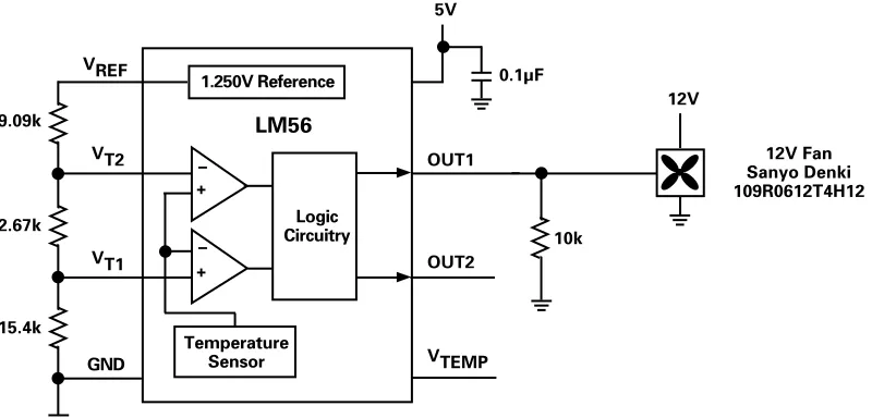
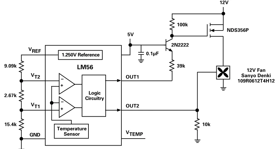
Simple Fan Controller
The circuit in Figure 5.1 senses system temperature and turns a cooling fan on when the sensors temperature exceeds a preselected value. The LM56 thermostat IC senses temperature and compares its sensor output volt-age to the voltvolt-ages at its VT1and VT2pins, which are set using three external resistors. The 1.25V system
volt-age reference is internal. As shown, VT1will go low and the fan will turn on when the sensors temperature
exceeds 50°C. If the sensors temperature rises above 70°C, VT2will go low. This output can be used to slow the system clock (to reduce processor power) or drive an interrupt that causes the microprocessor to initiate a shutdown procedure. If the second output isn’t needed, replace the 9.09k resistor with a short, and replace the 2.67k resistor with a 11.8k resistor. VT1will still go low at T=50°C, but VT2will remain inactive.
Typically, the LM56 will be located on the circuit board as close as possible to the microprocessor so that its temperature will be near that of the processor. This circuit is designed for a 12V fan. An alternative approach with a p-channel MOSFET and a 5V fan is shown in Figure 5.2
Figure 5.2. This circuit performs the same function as the circuit in 5.1, but it is designed for a 5V cooling fan.
Low/High Fan Controllers
The circuit in Figure 5.3 again uses the LM56, but in this case the fan is always on. When the circuit board’s temperature is low, the fan runs at a relatively slow speed. When temperature exceeds 50°C, the fan speed increases to its maximum value. As with the circuits in Figures 5.1 and 5.2, OUT2 is a second logic-level output that indicates that the LM56’s temperature is greater than 70°C. Again, if this second logic output is not need-ed, the VREFand VT2pins can be connected together and the two resistors replaced by a single resistor whose
value is equal to the sum of their resistances.
Another variation on this approach uses a MOSFET to turn the fan on at the lower temperature threshold, and the fan’s speed control input to increase the fan’s speed when the second threshold is exceeded.
[image:19.612.105.505.404.596.2]Figure 5.4. By combining the two approaches shown in the previous circuits, you can build a fan controller that turns the fan on at one temperature, then increases its speed if temperature rises above a second threshold.
Digital I/O Temperature Monitor
Figure 5.5. Place the LM75 near the microprocessor to monitor the microprocessors temperature in a mother-board application. Temperature data can be read at any time over the two-wire, I2Ccompatible serial interface. Up to 8 LM75s can share the same serial bus if their addresses are set to different values using A0, A1, and A2.
5.2 Interfacing External Temperature Sensors to PCs
LM75-to-PC interface
[image:21.612.129.483.48.287.2]The LM75 allows PCs to acquire temperature data through the parallel printer port with minimal circuitry as shown in Figure 5.6. The LM75 gets its power from a line on the parallel printer port. The jumpers on address pins A0, A1, and A2 allow you to select the LM75’s address. Up to eight LM75s can be connected to the same port and selected according to the chosen address.
Figure 5.6. PC-Based Temperature Acquisition via the Parallel Printer Port.
Pin 1 Pin
14
Pin 13 Pin
25
LSB
MSB addr+1
OS LM75
SDA SCL A0 A1 A2 8
3
1 2
4 C1 0.1 µF
SDA
SCL
2k
1N5712
7
5 Inside Personal Computer
6
addr
Read-Back Register
MSB LSB 2k
Isolated LM75-to-PC
You can couple an LM75 digital output temperature sensor through the isolated I2C interface shown in Figure 5.7. Electrically isolating the sensor allows operation in situations exposed to high common-mode voltages; or could be useful in breaking ground loops. Note that the SCL (clock) line is not bi-directional. The LM75 is a slave, and its SCL pin is an input only.
[image:22.612.66.565.164.624.2]The O.S. optocoupler is optional and needed only if it is desired to monitor O.S. Provide an isolated supply voltage, either a DC-DC converter or a battery. The LM75 will operate from 3V to 5V, and typically requires 250µA, while IC1 and IC3 require 7-10mA each (the LEDs require about 700µA, but only when active), for a total current drain of about 30mA.
Figure 5.7. Isolated PC-Based Thermometer.
3 LM75 6 5 4 Set As Desired AO A1 A2 OS SCL SDA 1 2 7 5V Supply All Optocouplers (IC1-IC5 HP HCPL2300 INT SDA SCL From Host Processor D1-D4 1N5712 0.1 8 Isolated 5V DC-DC Converter
hasten the battery discharge if the device is operating full-time. Therefore, the LM60 is shown here being pow-ered by a CMOS logic gate, which means that the LM60’s supply connection serves as the “shutdown” pin. Because temperature changes slowly, and can be measured quickly, the LM60 can be powered up for a small percentage of total operating time, say 1 second every 2 minutes, providing “quick” response to changes in temperature, but using only around 1µA average current.
Figure 5.8. 2.7V Temperature Sensor Operating From Logic Gate.
Battery Management
Battery charging circuits range in complexity from simple voltage sources with current-limiting resistors to sophisticated systems based on “smart batteries” that include microcontrollers, temperature sensors, ADCs, and non-volatile memory to store optimum charging data and usage history. The charge status of a battery is measured using terminal voltage and tracking the charge flowing in and out of the cells. Fast chargers for NiCad and NiMH batteries often also rely on cell temperature to help determine when to terminate charging.
In NiCad batteries, charging is an endothermic process, so a NiCad battery pack will either remain at the same temperature or cool slightly during charging. When the battery becomes overcharged, its temperature will begin to rise relatively quickly, indicating that the charging current should be turned off (see Figure 5.9a). Charging is an exothermic process in NiMH batteries, so temperature increases slowly during the entire charge cycle. In either kind of nickel-based battery, both voltage and temperature are often monitored to avoid dam-age from overcharging. However, in NiMH batteries the change in cell voltdam-age is much slower than in NiCd batteries, so temperature becomes the primary indicator of overcharging.
(a)
(b)
Figure 5.9. Typical NiCd Fast Charging Curves. Note that both cell voltage and cell temperature provide indica-tion of overcharging.
160 140 120 100 80 60 40 20 0 20 30 40 50 60
Charge (%C)
Cell Temperature (°C)
160 140 120 100 80 60 40 20 0 1.3 1.4 1.5 1.6
Charge (%C)
Cell Voltage
LM60
Logic device output
+VS
[image:23.612.167.451.357.700.2]“No Power” Battery Temperature Monitors
Figure 5.10 shows a temperature sensor housed in a battery pack for charge control and safety enhancement. The LM234 produces an output current that is proportional to absolute temperature (1µA/°K). This current can be converted to a voltage by connecting the LM234’s output to an external resistor, which is located in the host system, or in the battery charger, as shown here. With a 10kΩresistor, VTEMPis 10mV/°K. By using an external
FET to break the current path, current drain by the sensor drops to zero when temperature is not being moni-tored. Sensor current drain also drops to zero when the battery is unplugged from the charger, or when it is plugged into a charger that has no ac power, thus preventing accidental battery discharge.
Figure 5.10. This battery pack temperature sensor uses no power unless Q1 (located either in the charger, as shown here, or in the “load system”) is turned on. This helps prevent accidental battery discharge.
Figure 5.11 shows another “no power” battery pack temperature sensor circuit, this one using the LM235 two-terminal temperature sensor. The LM235 behaves like a two-two-terminal shunt voltage reference with a 10mV/°K temperature coefficient. A resistor to a positive voltage develops a current to power the LM235. In this circuit, the LM235 is in the battery pack, and the external resistor is in the charger. The LM235 operates at a nominal current of 1mA, and its output voltage (2.98V nominal at 25°C) drives an ADC. The resolution of the ADC depends on the desired sensitivity to temperature changes. With the 8-bit ADC shown here, 1LSB corresponds to 1°C change in temperature. The temperature range for accurate measurements is -23°C to +125°C. If more resolution is needed, a 10-bit converter will have a 1LSB transition every 0.25°C.
LM234
Battery Pack
VTemp 2 2 6
"Intelligent" Charger
To monitoring and control circuitry 10k
+
– R
1µA/°k
10mV/°k Q1
Figure 5.11. Voltage-Output Battery Pack Temperature Sensor
5.4 Audio
[image:25.612.87.519.508.687.2]Audio Power Amplifier Heat Sink Temperature Detector and Fan Controller
Figure 5.12 shows an overtemperature detector for power devices. In this example, an audio power amplifier IC is bolted to a heat sink and an LM35 Celsius temperature sensor is either glued to the heat sink near the power amplifier, or mounted on the printed circuit board on the opposite side from the heat sink (if the heat sink is mounted flat against one side of the printed circuit board. The comparators output goes low if the heat sink temperature rises above a threshold set by R1, R2, and the voltage reference. This fault detection output from the comparator now can be used to turn on a cooling fan. R3 and R4 provide hysteresis to prevent the fan from rapidly cycling on and off. The circuit as shown is designed to turn the fan on when heat sink temper-ature exceeds about 80°C, and to turn the fan off when the heat sink tempertemper-ature falls below about 60°C.
A similar circuit is shown in Figure 5.13. In this circuit, the sensor, voltage reference, and comparator are replaced by the LM56. The fan turns on at about 80°C, and the LM56’s built-in 5°C hysteresis causes the fan to turn off again when the sensors temperature drops below about 75°C.
Figure 5.12. In this typical monolithic temperature sensor application, sensor IC1 and its leads are attached to 60W audio power amplifier IC2’s heat sink. When the heat sinks temperature rises above the 60°C threshold temperature, comparator IC3’s output goes high, turning on the cooling fan.
LM35 IC1 Audio In +28V -28V +12V 10k 18k 10k 560k 10k 47k 1k 20k 3.3µF film 12V Fan LM3886 IC2 IC3 IC4 LM4041-1.2 LMC7211 Q1 NDS9410 10µF Thermally Connected R1* 1.1k R3 9.53k
Battery Pack "Intelligent" Charger Good Thermal Coupling LM335 IC1 *Choose for 1.35mA nominal current; see text Charging
Current Source
+5V
VREF+ COM CH1 CH0 +5V ADC10732 IC4 R4** **See Text
Choose for V0 near 4.5V IC2 LM4041-2.5 IC3 LM4041-1.2 To microcontroller +5V 8 2 0
R2 4 3 2
Figure 5.13. This circuit’s function is similar to that of the circuit above, except that the sensor, comparator, and voltage reference are integrated within the LM56. In this circuit, the fan turns on at 80°C and off at 75°C.
5.5 Other Applications
Two-Wire Temperature Sensor
When sensing temperature in a remote location, it is desirable to minimize the number of wires between the sensor and the main circuit board. A three-terminal sensor needs three wires for power, ground, and output signal; going to two wires means that power and signal must coexist on the same wires. You can use a two-terminal sensor like the LM334 or LM335, but these devices produce an output signal that is proportional to absolute temperature, which can be inconvenient. If you need an output signal proportional to degrees C, and you must have no more than two wires, the circuit in Figure 5.14 may be a good solution. The sensors output voltage is dc, and power is transmitted as an ac signal.
The ac power source for the sensor is a sine-wave oscillator (A1 and A2) coupled to the two-wire line through blocking capacitor C6. At the LM45 sensor, D1, D2, C1, and C3 comprise a half-wave voltage-doubler rectifier that provides power for the sensor. R2 isolates the sensors output from the load capacitance, and L1 couples the output signal to the line. L1 and C2 protect the sensors output from the ac on the two-wire line.
At the output end of the line, R3, L2, and C2 form a low-pass filter to remove ac from the output signal. C5 pre-vents dc current from flowing in R3, which would attenuate the temperature signal. The output should drive a high-impedance load (preferably 100kΩor greater).
Temperature Sensor +28V
-28V
+5V
20k
3.3µF film
5V Fan LM3886
IC2
Audio In 47k
1k
10µF
+
-8
7
6
5
LM56
GND VT1 VT2 VREF
Thermally Connected NDS356P
100k
MC05J3 COMAIR-ROTRON or
FBK04F05L Panasonic
R1 9.76K
R2 24k
IC1
1.250V Reference
VTEMP V+ 1
2
3
4
+
-Figure 5.14. This two-wire remote temperature sensor transmits the dc output of the sensor without reducing its accuracy.
4-to-20mA Current Transmitter (0°C to 100°C)
[image:27.612.113.500.49.388.2]This circuit uses an LM45 or LM35 temperature sensor to develop a 4-to-20mA current. The temperature sen-sors output drive is augmented by a PNP to drive a 62.5Ωload; this provides the 160µA/°C transfer function slope required to develop a 4-to-20mA output current for a 0°C to 100°C temperature range. The LM317 volt-age regulator and its load resistors draw about 2.8mA from the supply. The remaining 1.2mA is obtained by adjusting the 50Ωpotentiometer to develop an offset voltage on the temperature sensors ground pin.
Figure 5.15. 4-20mA Current Transmitter Temperature Sensor
V+
LM45
+
LM317
62.5 0.5%
4.7k
50 402 1% OUT
2N2907
OUT
ADJ IN
OFFSET ADJUST –
+6V to +10V +12
-12
LM45
+12
-12 R6
6.8k
R5 6.8k
R4 6.8k
R7 30k
R8 10k
C6 0.01µF
L2 100mH
C4
0.1µF 1µFC5 R3 1k Output
C2 0.1µF
Two-wire line C1
0.01µF
L1 100mH R2
1k C3
0.1µF
D2
D1
A1
A2 A1, A2 = LM6218
D1, D2 = 1N914
C8 200pF
C7 200pF C9
[image:27.612.162.444.517.678.2]Multi-Channel Temperature-to-Digital Converter
This circuit implements a low-cost system for measuring temperature at several points within a system and converting the temperature readings to digital form. With the components shown here, up to 19 LM45 temper-ature sensors drive separate inputs of an ADC08019 8-bit, 19-channel ADC with serial (microwire, SPI) data interface. The tiny SOT-23 sensor packages allow the designer to place the sensors in virtually any location within the system.
[image:28.612.131.481.207.611.2]The 1.28V reference voltage is chosen to provide a conversion scale of 1LSB=5mV=0.5°C, with full-scale equal to 128°C. The R-C network at the sensors’ outputs provide protection against oscillation if capacitive loads (or cables) may be encountered, and also help filter output noise. The reference voltage can be manually adjusted to 1.28V with the 10k potentiometer, or the potentiometer can be replaced with a fixed resistor. If 5% values will be used, a 3.3kΩresistor will work. For better accuracy, use 1% resistors; the pot can then be replaced by a 3.24kΩresistor.
Figure 5.16. 19-Channel Temperature-to-Digital Converter. Only one LM45 temperature sensor is shown. One
output of a voltage divider from the LM4040-4.1 voltage reference. With the divider components shown, the non-inverting input is at 3.48V, which is equal to the LM335’s output at 75°C. The amplifier has a gain of 100 to the difference between the measured temperature and the set-point.
[image:29.612.95.520.138.371.2]The output of A1 modulates the duty cycle of the oscillator built around comparator C1. When the oven is cold, the output of A1 is high, which charges the capacitor and forces C1’s output low. This turns on Q1 and delivers full dc power to the heater. As the oven temperature approaches the set-point, A1’s output goes lower, and adjusts the oscillators duty cycle to servo the oven temperature near the set-point.
Figure 5.17. 5V Oven Controller
Isolated Temperature-to-Frequency Converter
A simple way to transmit analog information across an isolation barrier is to first convert the analog signal into a frequency. The frequency can then easily be counted on the other side of the isolation barrier by a microcontroller. Figure 5.18 shows a simple way of implementing this. The LM45’s analog output, which is pro-portional to temperature, drives the input of an LM131 configured as a V-F converter. Over the temperature range of 2.5°C to 100°C, the LM45 produces output voltages from 25mV to 1V, which causes the LM131 to develop output frequencies from 25Hz to 1kHz.
Figure 5.18. Isolated Temperature-to-Frequency Converter
100k
LM45
+
LM131
GND
0.01µF
5k 12k
47 100k
7
6
1 2 4
Full Scale Adjust
8 5V
5.8k 1k
5
3
fOUT
1µF
0.01µF
Low Tempco 4N28 1M
6 1 9 300
10k
1.5k 1µF
LM4040 -4.1
LM335
6.8k A1 5V
100k
C1 100k
0.001
100k
5V 100k
5V
100k 2.7k
10k
2N5023 4.7µF SOLID TANTALUM
7 . 5 HEATER
THERMAL FEEDBACK
[image:29.612.101.498.494.688.2]6. Datasheets
Access National Semiconductor's temperature sensor
datasheets/pricing/demo board kits/free samples
via the internet!
http://www.national.com/catalog/sg2261.html
Or call your local
TL/H/6685
LM34/LM34A/LM34C/LM34CA/LM34D
Precision
Fahrenheit
Temperature
Sensors
December 1994
LM34/LM34A/LM34C/LM34CA/LM34D
Precision Fahrenheit Temperature Sensors
General Description
The LM34 series are precision integrated-circuit tempera-ture sensors, whose output voltage is linearly proportional to the Fahrenheit temperature. The LM34 thus has an advan-tage over linear temperature sensors calibrated in degrees Kelvin, as the user is not required to subtract a large con-stant voltage from its output to obtain convenient Fahren-heit scaling. The LM34 does not require any external cali-bration or trimming to provide typical accuracies ofg(/2§F at
room temperature andg1(/2§F over a fullb50 toa300§F temperature range. Low cost is assured by trimming and calibration at the wafer level. The LM34’s low output imped-ance, linear output, and precise inherent calibration make interfacing to readout or control circuitry especially easy. It can be used with single power supplies or with plus and minus supplies. As it draws only 75mA from its supply, it has very low self-heating, less than 0.2§F in still air. The LM34 is rated to operate over a b50§ to a300§F temperature range, while the LM34C is rated for ab40§ to a230§F range (0§F with improved accuracy). The LM34 series is available packaged in hermetic TO-46 transistor packages,
while the LM34C, LM34CA and LM34D are also available in the plastic TO-92 transistor package. The LM34D is also available in an 8-lead surface mount small outline package. The LM34 is a complement to the LM35 (Centigrade) tem-perature sensor.
Features
Y Calibrated directly in degrees Fahrenheit
Y Lineara10.0 mV/§F scale factor
Y 1.0§F accuracy guaranteed (ata77§F)
Y Rated for fullb50§toa300§F range
Y Suitable for remote applications
Y Low cost due to wafer-level trimming
Y Operates from 5 to 30 volts
Y Less than 90mA current drain
Y Low self-heating, 0.18§F in still air
Y Nonlinearity onlyg0.5§F typical
Y Low-impedance output, 0.4Xfor 1 mA load
Connection Diagrams
TO-46 Metal Can Package*
TL/H/6685 – 1 *Case is connected to negative pin (GND).
Order Numbers LM34H, LM34AH, LM34CH, LM34CAH or LM34DH See NS Package Number H03H
TO-92 Plastic Package
TL/H/6685 – 2
Order Number LM34CZ, LM34CAZ or LM34DZ See NS Package Number Z03A
SO-8
Small Outline Molded Package
TL/H/6685 – 20
Top View
N.C.eNo Connection
Order Number LM34DM See NS Package Number M08A
Typical Applications
TL/H/6685 – 3
FIGURE 1. Basic Fahrenheit Temperature Sensor (a5§toa300§F)
TL/H/6685 – 4
FIGURE 2. Full-Range Fahrenheit Temperature Sensor TRI-STATEÉis a registered trademark of National Semiconductor Corporation.
[image:31.612.114.524.93.686.2] [image:31.612.113.523.386.675.2]LM35/LM35A/LM35C/LM35CA/LM35D
Precision Centigrade Temperature Sensors
General Description
The LM35 series are precision integrated-circuit temperature sensors, whose output voltage is linearly proportional to the Celsius (Centigrade) temperature. The LM35 thus has an advantage over linear temperature sensors calibrated in ˚ Kelvin, as the user is not required to subtract a large con-stant voltage from its output to obtain convenient Centigrade scaling. The LM35 does not require any external calibration or trimming to provide typical accuracies of±1⁄4˚C at room temperature and±3⁄4˚C over a full −55 to +150˚C tempera-ture range. Low cost is assured by trimming and calibration at the wafer level. The LM35’s low output impedance, linear output, and precise inherent calibration make interfacing to readout or control circuitry especially easy. It can be used with single power supplies, or with plus and minus supplies. As it draws only 60 µA from its supply, it has very low self-heating, less than 0.1˚C in still air. The LM35 is rated to operate over a −55˚ to +150˚C temperature range, while the LM35C is rated for a −40˚ to +110˚C range (−10˚ with im-proved accuracy). The LM35 series is available packaged in
hermetic TO-46 transistor packages, while the LM35C, LM35CA, and LM35D are also available in the plastic TO-92 transistor package. The LM35D is also available in an 8-lead surface mount small outline package and a plastic TO-220 package.
Features
n Calibrated directly in ˚ Celsius (Centigrade) n Linear + 10.0 mV/˚C scale factor n 0.5˚C accuracy guaranteeable (at +25˚C) n Rated for full −55˚ to +150˚C range n Suitable for remote applications n Low cost due to wafer-level trimming n Operates from 4 to 30 volts n Less than 60 µA current drain n Low self-heating, 0.08˚C in still air n Nonlinearity only±1⁄4˚C typical
n Low impedance output, 0.1Ωfor 1 mA load
Typical Applications
[image:32.612.107.516.248.680.2]DS005516-3
FIGURE 1. Basic Centirade Temperature Sensor (+2˚C to +150˚C)
DS005516-4
Choose R1= −VS/50 µA
VOUT=+1,500 mV at +150˚C
= +250 mV at +25˚C = −550 mV at −55˚C
FIGURE 2. Full-Range Centigrade Temperature Sensor September 1997
LM35/LM35A/LM35C/LM35CA/LM35D
Precision
Centigrade
T
emperature
TL/H/11754
LM45B/LM45C
SOT-23
Precision
Centigrade
Temperature
Sensors
May 1995
LM45B/LM45C
SOT-23 Precision Centigrade Temperature Sensors
General Description
The LM45 series are precision integrated-circuit tempera-ture sensors, whose output voltage is linearly proportional to the Celsius (Centigrade) temperature. The LM45 does not require any external calibration or trimming to provide accu-racies ofg2§C at room temperature andg3§C over a full b20 toa100§C temperature range. Low cost is assured by
trimming and calibration at the wafer level. The LM45’s low output impedance, linear output, and precise inherent cali-bration make interfacing to readout or control circuitry espe-cially easy. It can be used with a single power supply, or with plus and minus supplies. As it draws only 120mA from its supply, it has very low self-heating, less than 0.2§C in still air. The LM45 is rated to operate over ab20§toa100§C temperature range.
Applications
Y Battery Management
Y FAX Machines
Y Printers
Y Portable Medical Instruments
Y HVAC
Y Power Supply Modules
Y Disk Drives
Y Computers
Y Automotive
Features
Y Calibrated directly in§Celsius (Centigrade)
Y Lineara10.0 mV/§C scale factor
Y g3§C accuracy guaranteed
Y Rated for fullb20§toa100§C range
Y Suitable for remote applications
Y Low cost due to wafer-level trimming
Y Operates from 4.0V to 10V
Y Less than 120mA current drain
Y Low self-heating, 0.20§C in still air
Y Nonlinearity onlyg0.8§C max over temp
Y Low impedance output, 20Xfor 1 mA load
Connection Diagram
SOT-23
TL/H/11754 – 1
Top View
See NS Package Number M03B (JEDEC Registration TO-236AB)
SOT-23 Order Device
Number Marking Supplied As
LM45BIM3 T4B 250 Units on Tape and Reel LM45BIM3X T4B 3000 Units on Tape and Reel LM45CIM3 T4C 250 Units on Tape and Reel LM45CIM3X T4C 3000 Units on Tape and Reel
Typical Applications
TL/H/11754 – 3
FIGURE 1. Basic Centigrade Temperature Sensor (a2.5§C toa100§C)
TL/H/11754 – 4
Choose R1e bVS/50mA VOUTe(10 mV/§CcTemp§C)
VOUTe a1,000 mV ata100§C
e a250 mV ata25§C e b200 mV atb20§C
FIGURE 2. Full-Range Centigrade Temperature Sensor (b20§C toa100§C)
[image:33.612.117.532.90.701.2]