A NUMERICAL MODELING OF A VARIABLE CONDUCTANCE
THERMOSYPHON BY USE OF A BINARY MIXTURE
H. Shokohmand
Department of Mechanical Engineering, Tehran University Tehran, Iran, [email protected]
A. Hassani
Branch of Science and Research, Islamic Azad University Tehran, Iran, [email protected]
(Received: November 19, 2001 – Accepted in Revised Form: October 10, 2002)
Abstract In this paper the steady state performance of a variable conductance heat pipe, which its
working fluid consists of two components (R11+ R113) is modeled. The role of the liquid film momentum and axial normal stresses are considered by use of the mean property of mixture and the governing equations are solved by conventional numerical methods. The results of the present model have been compared with other numerical models and experimental works done by other investigators. The model presented could be used for optimization studies and design of variable conductance thermosyphons.
Key Words Thermosyphon, Variable Conductance, Binary Mixture
ﻩﺪﻴـﻜﭼ
ﻩﺪﻴـﻜﭼ
ﻩﺪﻴـﻜﭼ
ﻩﺪﻴـﻜﭼ
ﻥﻮﻔﻴﺳﻮﻣﺮﺗﺕﺭﺍﺮﺣﻪﻟﻮﻟﻚﻳﻢـﺋﺍﺩﺩﺮـﻜﻠﻤﻋ،ﻪـﻟﺎﻘﻣﻦـﻳﺍﺭﺩ
ﻱﺍﺭﺍﺩ ﺩﺮﺒﻣﻭﺩﺯﺍﻲﻃﻮﻠﺨﻣ
R11
ﻭ
R113
ﻥﺍﻮﻨـﻋﻪـﺑ
ﻞﻣﺎﻋﻝﺎﻴﺳ
ﺖﺳﺍﻪﺘﻓﺮﮔﺭﺍﺮﻗﻲﺳﺭﺮﺑﺩﺭﻮﻣ
.
ﻣﺕﻼﻣﺎﻌﻣ
ﺑﻲﮕﺘﺳﻮﻴﭘﻭﻱﮊﺮﻧﺍ،ﻡﻮﺘﻨﻤ
ﺭﺩﺎﺑﻭﻥﺎﻣﺰﻤﻫﺭﻮﻄ
ﻮﺧﺯﺍﻩﺩﺎﻔﺘﺳﺍﺎﺑﻭﻥﺎﻳﺮﺟﺭﺩﻱﺭﻮﺤﻣﻱﺩﻮﻤﻋﻱﺎﻫﺶﻨﺗﻦﺘﻓﺮﮔﺮـﻈﻧ ﺍ
ﺨﻣﻂﺳﻮﺘﻣﺹ ﺑﻁﻮﻠ
ﻩﺪﺷﻞﺣﻱﺩﺪﻋﺭﻮﻄ
ﺖﺳﺍﻪﺘﻓﺮﮔﺭﺍﺮﻗﻞﻴﻠﺤﺗﻭﻪﻳﺰﺠﺗﺩﺭﻮﻣﻪﻟﻮﻟﺮﻴﻐﺘﻣﺖﻳﺍﺪﻫﺭﺎﺘﻓﺭﻭ
. ﻭﻱﺩﺪﻋﻱﺎﻫﻝﺪﻣﺎﺑﻝﺪﻣﻦﻳﺍﺯﺍﻞﺻﺎﺣﺞﻳﺎﺘﻧ
ﺖﺳﺍﻪﺘﻓﺮﮔﺭﺍﺮﻗﻲﺳﺭﺮﺑﺩﺭﻮﻣﻝﺪﻣﺕﻮﻗﻭﻒﻌﺿﻁﺎﻘﻧﻭﻩﺪﺷﻪﺴﻳﺎﻘﻣﻦﻴﻘﻘﺤﻣﺮﮕﻳﺩﻲـﺑﺮﺠﺗﺞﻳﺎﺘـﻧ
.
ﺮﺿﺎﺣﻝﺪﻣ
ﻮﻟﻲﺣﺍﺮﻃﻭﻱﺯﺎﺳﻪﻨﻴﻬﺑﺕﺎﻌﻟﺎﻄﻣﺭﺩﺪﻧﺍﻮﺗﻲﻣ ﺮﻴﻐﺘﻣﺖﻳﺍﺪﻫﻉﻮﻧﺯﺍﻥﻮﻔﻴﺳﻮﻣﺮﺗﻱﺎﻫﻪﻟ
ﺩﻮﺷﻩﺩﺮﺑﺭﺎﻜﺑ
.
1. INTRODUCTION
For the first time Katzof [1] noted that small amounts of non-condensable gas can provide a simple thermostatic control for heat pipes. Since then, extensive efforts have been done for better understanding of gas loaded device performance and creating their useful constant temperature behavior. With gas loading, increasing the power input raises the system pressure, which compresses the non-condensable gas accumulated at the end of the condenser. This leads to an increase in condenser surface area and controls the evaporator temperature increase [2-5].
Recently Hijikata et al. [6] found that a similar variable conductance behavior could occur in reflux thermosyphons, even without non-condensable
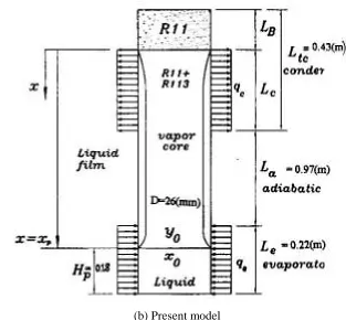
gases, when the thermosyphon evaporator is charged with a liquid pool of R113 and R11. With this binary mixture, a shut-off zone was observed at the end of the condenser, as illustrated schematically by Figure l(a). By this binary mixture, one can increase and decrease the shut-off zone by decreasing and increasing the input power to the evaporator, respectively. It is important to note that this variable conductance behavior is not extendable for all binary mixtures.
their model did not account for the shut-off zone of the condenser. As illustrated in Figure 1(a), modeling of a two- phase closed thermosyphon requires a fundamental understanding of the following interrelated physical processes:
- Heat transmission through the evaporator wall. - Boiling in the evaporator region (both liquid
pool and liquid film).
- Condensation in the condenser region. - Heat conduction through the condenser wall. - Movement of the vapor core and the liquid film. Compared with the wicked heat pipe, thermosyphon transients in wickless pipes occur much faster, because of the thermal response delay to heat transfer introduced by the wetted wick [6]. This is the main reason we used the wickless thermosyphon for the present analysis. Steady state performance of a variable conductance thermosyphon is the focus of this work.
A comprehensive model is developed from the basic conservation laws, and numerical techniques are developed to solve the nonlinear governing
equations.
The liquid-film momentum and normal stress, which have not been considered in previous studies, are included in this paper. From The results of this model, most operation parameters such as the mean vapor temperature, liquid film thickness, mass fluxes, as well as the operating limits (dry- out and flooding) associated with the steady state performance could be predicted. The predictions of the present model have been compared with numerical and experimental results of other investigators.
2. NUMERICAL MODEL AND MODEL ASSUMPTIONS
In the present numerical model Figure 1(b), the following assumptions used:
- The vapor and liquid flows are considered one dimensional, steady and Newtonian fluid. - Compressibility of the vapor is negligible. (a) Actual model (b) Present model
- The vapor and liquid binary mixture are in equilibrium on the phase equilibrium diagram as an ideal mixture (Raoult’s law).
- Pressure drop in the liquid film is negligible. - The axial conduction and the viscous dissipation
are negligible.
- Concentration of the vapor from the top boiling pool surface till condenser entrance is nearly constant.
- Effect of diffusion at the interface of the two regions (effective and non-effective length of the condenser) is negligible.
- The film thickness, compared with the pipe radius is negligible. (δ/R<<1).
3. CONTINUITY AND MOMENTUM EQUATIONS OF LIQUID FILM
The continuity and momentum equations of the liquid film could be written as:
[
]
2
RV
dx
u
)
r
R
(
d
L 2 2=
−
(1)0
R
2
r
2
g
)
r
R
(
dx
du
3
4
)
r
R
(
dx
d
]
u
)
r
R
[(
dx
d
i L 2 2 L L 2 2 2 L 2 2 L=
τ
+
τ
+
ρ
−
−
−
µ
−
−
ρ
ω (2) In Equation 2, the first term corresponds to thetotal momentum change (including momentum advection) and the second term accounts for the axial normal stress in the liquid film. The final three terms corresponds to gravity, wall shear stress and interfacial shear stress, respectively. Unlike the pervious studies, the momentum advection contribution and the normal stress terms are included. Both of these terms affect thermosyphon performance. The normal stress term is also important in the numerical solution procedure.
The wall shear stress and the interfacial shear stress are modeled as:
i w f 2 L v v i f 2 L L
w (u u ) C
2 1 C
u 2
1ρ τ = ρ +
= τ
(3)
where uv and uL are both positive in magnitude but opposite in direction. Friction coefficients could be written as [8]:
el w
R
16
Cf
=
(Laminar liquid film, ReL<2040) (4)4 / 1 e w
0
.
079
R
1Cf
=
− (Turbulent liquid film, ReL>2040)(5)
1
e
R
16
Cf
el i−
ψ
=
ψ (Laminar vapor core,ReL < 2040) (6)
w here • is a correction factor accounting for the
effects of phase change[8]:
v L
4
VR
µ
ρ
−
=
ψ
1525
R
Cf
33 . 0 e i v=
(Transition region 2040<Rev<4000)(7) 2 X 1 i
R
X
05
.
0
Cf
δ
+
=
(Turbulent vapor core
R
ev≥
4000
) (8)where
=
BO 07 . 9 2 X1
10
2
BO
2574
.
0
X
andBO
74
.
4
63
.
1
X
2=
+
.4. MASS AND ENERGY EQUATIONS FOR LIQUID FILM AND VAPOR
Assuming that the conduction and convection heat transfer at the liquid-vapor interface inside the thermosyphon are much smaller than the transport of latent heat from phase change, the energy equation for liquid film flow could be written as:
L fg w s fg L
h
)
T
T
(
h
h
q
V
ρ
−
=
ρ
′′
where the film heat transfer coefficient from energy balance is defined as [8]:
)
T
T
(
)
T
T
(
K
h
w s w i L−
δ
−
=
(Laminar,R
el≤
2040
) (10)3 1 2 L L 3 1 r 5 1 e ) g ( K P R 056 . 0 h L ν = −
(Turbulent, Rel>2040) (11)
For the upward vapor core flow, the continuity equation can be written as:
RV
2
dx
)
u
r
(
d
L v 2v
=
ρ
ρ
(12)Combining Equation 12 with the Equation 1, one can write:
[
]
dx
)
u
r
(
d
dx
u
)
r
R
(
d
v 2 v L 2 2L
=
ρ
−
ρ
(13)or in integrated form:
v 2 v L 2 2
L
(
R
−
r
)
u
=
ρ
r
u
ρ
(14)During steady-state operation, the relationship in Equation 14 implies that the downward mass flow rate of liquid film equals the upward mass flow rate at each cross section of the thermosyphon. From the Equation 14, the vapor core velocity can be evaluated as:
L 2 2 2 v L v
u
r
r
R
u
−
ρ
ρ
=
(15)Due to the assumptions made so far, it is not necessary to include momentum and energy equations for the vapor core. For the liquid pool surface, the continuity and energy equations are:
(
)
vp2 p v LP 2 p 2
L
R
−
r
u
=
ρ
r
u
ρ
(16)(
)
vp fg2 p v p "
e
2
RH
r
u
h
q
&
=
ρ
(17)Equation 16 and 17 imply that the mass and energy flowing into the liquid pool are equal to those flowing out of the liquid pool.
The boundary conditions for uL and r are as
follows:
- At the top end of the thermosyphon, (x = 0):
0
u
,
R
r
=
L=
(18)- At the liquid pool surface (x = x
p), from
Equations 16 and 17 one can write:
[
]
fg p Lp 2 p Lh
)
RH
2
(
q
u
r
R
−
=
′′
ρ
&
(19)In addition to these basic equations and boundary conditions, relations for the overall conservation of mass and energy in the entire thermosyphon system are also needed for calculating the liquid pool depth and determining the mean vapor temperature. The respective equations are:
[
]
∫
π
ρ
+
π
−
ρ
+
ρ
π
=
xP0 L 2 2 v 2 L P 2
dx
)
r
R
(
r
H
R
M
(20)∫
c−
=
∫
e−
a
x
0
x
x we s
wc
s
T
)
dx
h
(
T
T
)
dx
T
(
h
(21)where the heat transfer h in the liquid pool is modeled as [8]:
4 . 0 " e atm 1 . 0 L 4 . 0 fg 25 . 0 v 2 . 0 7 . 0 p 3 . 0 L 65 . 0 L
)
q
)(
P
P
(
h
g
C
K
32
.
0
h
&
µ
ρ
ρ
=
(22)By use of phase equilibrium diagram, Raoult’s law and vapor pressure curve of each component, the mass fraction of the liquid pool and vapor core are calculated as follows [9]:
F
P
P
P
P
x
B A B 11 R
−
−
F
P
X
P
y
A R1111
R
=
(24)where F is the ratio of the molecular weight of R11 to mixture molecular weight.
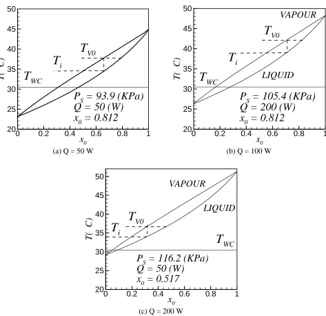
In Figure 2 a typical phase equilibrium diagram based on mass fraction of R 113 is shown.
5. CONDNSER EFFECTIVE LENGTH
As illustrated in Figure 1(b), the present model is based on the separation of the non-condensable region (more volatile component), from the active region of the condenser. This is the reason of neglecting the diffusion of two components at the boundary of the two regions. By this assumption, effective condenser length is approximated as:
0 0.2 0.4 0.6 0.8 1
x
020 25 30 35 40 45 50
T(
C)
P
S= 93.9 (KPa)
Q = 50 (W)
x
0= 0.812
T
V0T
iT
WC0 0.2 0.4 0.6 0.8 1
x
020 25 30 35 40 45 50
T(
C
)
P
S= 105.4 (KPa)
Q = 200 (W)
x
0= 0.812
T
V0T
iT
WCLIQUID
VAPOUR
(a) Q = 50 W (b) Q = 100 W
0 0.2 0.4 0.6 0.8 1
x
020 25 30 35 40 45 50
T(
C
)
P
S= 116.2 (KPa)
Q = 50 (W)
x
0= 0.517
T
V0T
iT
WCLIQUID
VAPOUR
(c) Q = 200 W
B tc
ceff
L
L
L
=
−
(25)where LB is the length occupied by the more
volatile component, which in steady state conditions acts as a blocked length for exchanging the heat at condenser.
The mixture vapor of R11+ R113 with vapor concentration of yo enters to the condenser zone.
With decreasing mixture temperature, it becomes liquid at the interface temperature and total pressure (PS). In this way, concentration of more
volatile component increases and it accumulates at the interface and the end of the condenser as a blocked length (Figure 1(a)).
In the present model we have assumed that the entire more volatile component (non-condensable) is stored at non- effective length of the condenser (LB) as shown in Figure 1(b).
6. NUMERICAL SOLUTION METHOD
Before solving the momentum and energy equations, mean vapor temperature and system pressure are assumed known. Then using the vapor pressure table for each component and Raoult’s law, the mass concentration in liquid (xo) and
vapor (y0) are calculated. Continuity and
momentum equations have been discretized by use of finite difference scheme, on an orthogonal grid. By a known value of pool depth of liquid and assuming the values of non-effective length of the condenser, condenser temperature and evaporator temperature, starting from the first effective point of condenser (uL = 0), momentum and energy
equations are solved for the velocity at the second point.
The mean velocity of the vapor is calculated by use of Equation 15, ReL, Rev, and drag coefficients
(Cfi, Cfw) are calculated by Equation 20. From the
above results, wall and interface shear stresses are found. Finally after substitution of the above five terms in Equation 20, by increasing or decreasing the film thickness (for condenser or evaporator) satisfaction of Equation 2, (sum of terms must be zero) is checked. Knowing the film thickness of the first point and assumption of film thickness for
next point the procedure is continued till final point at the end of condenser. Finally the first guess of non-effective length at end of condenser is checked by use of Equation 14. Along the adiabatic length, film thickness of the liquid, film velocity and vapor core velocities are constant. The foregoing procedure is repeated for evaporator section by reduction of the film thickness. By calculation of heat of each element along the condenser, total heat removal from condenser (or input to evaporator) is found and by use of film and pool boiling heat transfer coefficients, balance of Equation 21 is checked. If the desirable balance didn’t satisfy, the procedure will be repeated by changing the mean temperature of the vapor. After balance of energy Equation 21, the real amount of pool depth (Hp) is checked by use of Equation 19.
If the difference between the first guess and the calculated pool depth becomes more than five percent, the program starts again with a new guess calculating the vapor mass, liquid mass and total mass of the mixture. The following equation is used for determining the average interface temperature along the condenser:
S
i 0 P P
T T
i
y
x
==
= (26)In all calculations, the mean property of the mixture based on mass percent of liquid and vapor is applied. This model can also predict two important operating limits such as dry-out and flooding.
During the program execution one must note that the first guessed values must not lead to the flooding on interface and dry-out in the evaporator. Physically, flooding implies that the local shear stress on the liquid film is larger than the gravitational force.
The resulting net upward force retards the down- ward liquid- film flow and results in an unstable flow pattern.
7. COMPARISONS AND DISCUSSION OF RESULTS
The relationship between the temperature and concentration is shown in the phase equilibrium diagram (Figure 2) where Ti denotes the average
interfacial temperature weighted by condensation mass flux. y0 and x0 are specified at the saturated
concentration. xi is nearly equal to y0 because the
vapor that enters the cooling section condenses
completely. Raoult’s law has been applied for calculating the results shown in this figure.
Therefore the maximum temperature difference in the vapor phase (Tv0-Ti), is roughly given by the
temperature difference between the saturated vapor and liquid line at y0. Typical equilibrium diagrams for four conditions are shown in Figures 2(a, b, c). Mean vapor temperature and block length (occupied by R11) are shown in Figure 3(a, b). As expected, by increasing the pressure (or inlet vapor temperature), non-effective block length is reduced and for the values of power more than 100 (watt) this length is nearly zero.
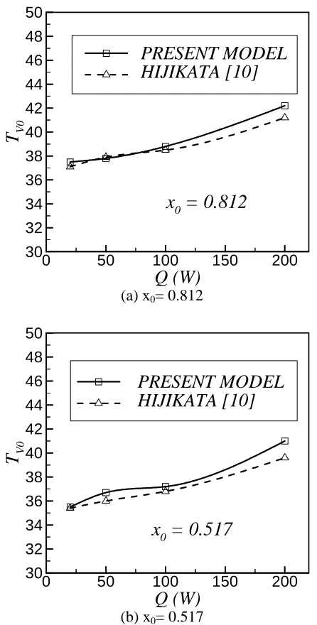
Results for two different liquid concentrations, namely 0.812 and 0.512 are shown In Figures 4(a, b). Inlet temperature of vapor versus power of the thermosyphon pipe for these two concentrations are shown and compared with Hijiakta numerical model [10].
As shown in the diagram of, Figure 4(a) at high concentrations, agreement between the two models is better in comparison with the low concentration. In Figure 4(b) this effect is shown clearly.
One must note that in all power levels, the prediction of the present model has a steady temperature higher than Hijikata numerical model [10]. This is due to the absence of diffusion between the interface of active and non-active lengths and neglecting of heat exchanged between the two zones. This effect will be dominant with increasing the power and therefore we have a higher steady pipe temperature.
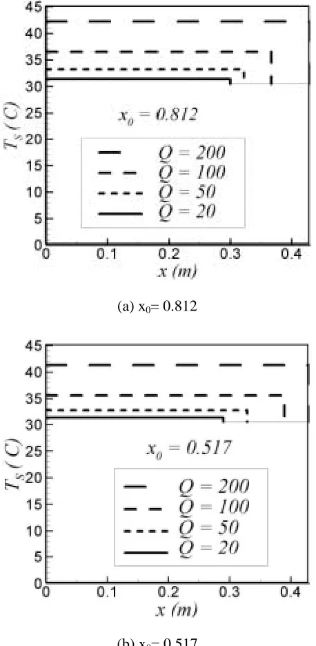
By increasing the inlet vapor temperature, effect of diffusion will be negligible because the system pressure reduces the block length, but in low inlet vapor temperature this effect will be very important (Figure 5).
For powers more than 50(w), the non-effective length that calculated by this model has a relatively good agreement with HIJIKATA model [10]. At low power the difference between the two models is relatively high. Finally, the calculated results are compared with the previous experimental result [10]. Figure 6(a) shows the comparison of the overall temperature difference in the cooling section, (Tv0-Twc), in which the theoretical values
for the condensation of pure vapor (R113 and R11) are also shown by dotted lines. Although the agreement between the present analysis and experimental results is not perfect, the constant
0 50 100 150 200
Q (W)
30 32 34 36 38 40 42 44 46 48 50
T
V0PRESENT MODEL
HIJIKATA [10]
x
0= 0.812
(a) x0= 0.812
0 50 100 150 200
Q (W)
30 32 34 36 38 40 42 44 46 48 50
T
V0PRESENT MODEL
HIJIKATA [10]
x
0= 0.517
(b) x0= 0.517
temperature behavior in the case of binary mixture is well predicted when compared to the condensation of pure vapors.
In addition, the predicted system pressure of present analysis agrees with other experimental and numerical results [10] as shown in Figure 6(b). Effect of diffusion at high concentration leads to an
0 0.05 0.1 0.15
LB 37
38 39 40 41 42 43
TV0
PRESENT MODEL HIJIKATA [9]
x0= 0.812
TWC= 30.5
Figure 5. Variation of vapor temperature versus non-effective length.
(a) Overall temperature difference
(b) System pressure
Figure 6. Comparison with experimental results. (a) x0= 0.812
(b) x0= 0.517
increase in effective condenser surface area and the related temperature difference reduction shown in the figure.
The present analysis neglects such detailed aspects as the effect of interfacial waves on liquid film, turbulence in the inlet vapor flow, and the distribution of velocity, temperature and concentration in the inlet vapor due to the existence of adiabatic section. These effects should be incorporated for more accurate analysis, however, the present model gives an understanding of the essential features of condensation phenomena in the cooling and heating sections. It also provides a practical method of prediction, to a certain degree of accuracy without requiring the detailed information on flow structures to be available
8. CONCLUSIONS
Condensation heat transfer in the cooling and heating sections of a binary heat pipe was analyzed numerically, and the following conclusions were obtained:
1. In the case of large heat loads, condensation occurs in the whole cooling section, in which case the vapor inlet temperature increases with increasing in heat load, which corresponds to an increase in the system pressure.
2. In the case of small heat loads, a non-condensing region appears which its length changes with a variation of heat load. In this case blocked condenser length, and the limiting temperature difference in the phase equilibrium diagram give the lower limit of the overall temperature difference, resulting in a constant temperature behavior.
3. Although the present analysis could predict the experimental data, further developments should be made to include the effects of diffusion at the interface of effective and non-effective lengths in cooling section.
9. NOMENCLATURE
Bo Bond number (4 gR )
2 l
σ ρ
Cf Friction Coefficient
CPL Liquid specific heat
dx Grid size
F Ratio of molecular weights
(
M
R11/
M
mix)
g Gravitational accelerationh Heat transfer coefficient hfg Latent heat of vaporization
HP Depth of liquid pool
KL Liquid thermal conductivity
L Length of thermosyphon M Total amount of working fluid P Partial pressure
PS Total pressure of system
Pr Liquid Prandtl number
q
&
′′
Wall heat fluxQ Power of Pipe
R Inner radius of thermosyphon r Vapor core radius
Re Reynolds number
(
4
Γ
/
µ
)
T TemperatureTS Saturated temperature
u Velocity
V Vapor condensation x Axial distance from the top of y Vapor mass concentration
Greek Symbols
Γ
Liquid mass flow rate per meter `δ Liquid film thickness
µ
Dynamic viscosityν
Kinematic viscosityρ
Densityσ
Liquid surface tensionτ
Shear stressψ
Phase change correction factorSubscripts
a Adiabatic region
atm Atmospheric inside the thermosyphon c Condenser region
e Evaporator region i Phase interface L Liquid phase P Liquid pool surface
c
L
Total length of condenser S Saturationw Tube wall V Vapor phase
t Total
A More volatile component (R11) velocity, volume B Less volatile component (R113)
0 Pool condition the liquid film, liquid mass concentration
10. REFERENCES
1. Katzoff, S., “Heat Pipes and Vapor Chambers for Thermal Control of Spacecraft: Thermophyics of Spacecraft and Planetary Bodies”, (Edited by G. B. Heller), Academic Pub., New York, (1947), 225-234. 2. Edwards, D. K. and Marcus, B. D., “Heat and Mass
Transfer in the Vicinity of the Vapor-Gas Front in a Gas Loaded Heat Pipe”, Journal of Heat Transfer, Vol. 94, Ser. C, No. 2, (1972), 155-162.
3. Hijikata, K., Chen, S. J. and Tien, C. L., “Non-Condensable Gas Effect on Condensation in a Two-Phase Closed Thermosyphon”, International Journal of Heat and Mass Transfer, Vol. 27, No. 8, (1984), 1319-1325.
4. Bobco, R. P., “Variable Conductance Heat Pipes: a First Order Model”, Journal of Thermophysics and Heat Transfer, Vol. 1., No. 1, (1987), 35-42.
5. Peterson, P. F. and Tien, C. L. “Numerical and Analytical Solutions for Two Dimensional Gas Distribution in Gas-Loaded Heat Pipes”, Journal of Heat Transfer, Vol. 111, (1989), 598-604.
6. Hijikata, K., Hasegawa, H. and Nagasaki, T., “A Study on a Variable- Conductance Heat Pipe Using a binary Mixture”, Proceeding of the XXth. International Symposium of the International Center for Heat and Mass Transfer, Hemisphere, New York, (1988). 7. Tien, C. L., Rohani, A. R., “Theory of Two Component
Heat Pipes”, Journal of Heat Transfer, Vol. 94, Ser. C, No. 4, (1972), 479-484
8. Zuo, Z. J. and Gunnerson, F. S., ”Numerical Modeling of the Steady State Two- Phase Closed Thermosyphone”, Int. J. of Heat and Mass Transfer, Vol. 37, No. 17, (1994), 2715- 2722.
9. McCabe, L. and Smith, C., “Unit Operations of Chemical Engineering”, Third Edition, New York, (1983).