Behavior of Packed Bed Thermal Storage

(1)

RESEARCH NOTE

BEHAVIOR OF PACKED BED THERMAL STORAGE

F. A. Hessari, S. Parsa and A. K. Khashechi

Materials and Energy Research Center

P. O. Box 14155-4777, Tehran, Iran, F_A_Hessari@yahoo.com

(Received: September 21, 2003 – Accepted in Revised Form: February 2, 2004)

Abstract A packed bed thermal storage has several desirable characteristics to be used for energy storage. The behavior of packed bed is predicted by set of differential equations. A numerical solution is developed for packed bed storage tank accounting to the secondary phenomena of thermal losses and conduction effect. The effect of heat loss to surrounding (k1), conduction effect (k2) and air

capacitance (k3) are examined in the numerical solution. It is found that the values of k1 and k2 are

small and can practically be neglected in the solution. The solution indicates the profiles of air and rock bed temperatures with respect to time and length of the bed.

Key Words Packed Bed; Storage Tank; Numerical Solution, Heat Loss

ﻩﺪﻴﻜﭼ

ﺭﺩ ﻩﺩﺎﻔﺘﺳﺍ ﻱﺍﺮﺑ ﻲﺒﺳﺎﻨﻣ ﻲﻜﻴﻧﺎﻜﻣ ﻭ ﻲﻜﻳﺰﻴﻓ ﺹﺍﻮﺧ ﻱﺍﺭﺍﺩ ﺖﺑﺎﺛ ﺮﺘﺴﺑ ﻉﻮﻧ ﺯﺍ ﺎﻣﺮﮔ ﻩﺮﻴﺧﺫ ﻊﺒﻨﻣ

ﺖﺳﺍ ﻲﻳﺎﻣﺮﮔﻩﺮﻴﺧﺫﻱﺎﻬﻤﺘﺴﻴﺳ

. ﺶﺑﺎﺗﻭﺯﻭﺭﺕﺎﻋﺎﺳﺭﺩ ﺖﻳﺩﻭﺪﺤﻣﻞﻴﻟﺩﻪﺑ ﻱﺪﻴﺷﺭﻮﺧﻲﺸﻳﺎﻣﺮﮔﻱﺎﻬﻤﺘﺴﻴﺳ

ﻴﺧﺫﻢﺘﺴﻴﺳﻲﻋﻮﻧﻱﺍﺭﺍﺩﺪﻳﺎﺑﺪﻴﺷﺭﻮﺧﺭﻮﻧ

ﺪﻨﺷﺎﺑﺎﻣﺮﮔﻩﺮ

. ﻲﻜﻴﻣﺎﻨﻳﺩﻭﻲﺗﺭﺍﺮﺣ،ﻲﻜﻴﻧﺎﻜﻣﻱﺎﻫﺭﺎﺘﻓﺭﻖﻴﻘﺤﺗﻦﻳﺍﺭﺩ

ﺩﺭﻮﻣﺕﺭﺍﺮﺣﻭﻡﺮﺟﻝﺎﻘﺘﻧﺍﻞﻴﺴﻧﺍﺮﻔﻳﺩﺕﻻﺩﺎﻌﻣﺯﺍﻱﺍﻪﻋﻮﻤﺠﻣﻪﻠﻴﺳﻮﺑﺍﺭﺖﺑﺎﺛﺮﺘﺴﺑﻉﻮﻧﺯﺍﻲﻳﺎﻣﺮﮔﻩﺮﻴﺧﺫﻢﺘﺴﻴﺳ

ﺵﻭﺭﺯﺍﻦﻴﻨﭽﻤﻫﻭﻩﺩﺍﺩﺭﺍﺮﻗﻪﻌﻟﺎﻄﻣ

Finite Element

ﻲﻣﻩﺩﺎﻔﺘﺳﺍﺕﻻﺩﺎﻌﻣﻦﻳﺍﻞﺣﻱﺍﺮﺑ ﺩﻮﺷ . ﺍﺮﺿﺮﺛﺍ ﺖﺑﺎﺛﺐﻳ k1 ، k2 ﻭ k3

ﺖﺳﺍﻩﺪﺷﻲﺳﺭﺮﺑﺕﻻﺩﺎﻌﻣﻦﻳﺍﻞﺣﺭﺩ

. ﺐﻳﺍﺮﺿﺭﺍﺪﻘﻣﻪﻛﺖﺳﺍ ﻩﺪﺷﻱﺮﻴﮔﻪﺠﻴﺘﻧ

k1 ﻭ

k2 ﺭﺩﻱﺮﺛﺍ

ﺩﺭﺍﺪﻧﺖﺑﺎﺛﺮﺘﺴﺑﻲﻜﻴﻣﺎﻨﻳﺩﺭﺎﺘﻓﺭﻲﻳﻮﮔﺶﻴﭘﻭﺕﻻﺩﺎﻌﻣﻞﺣ

.

1. INTRODUCTION

The limited amount of fossil energies has forced scientists all over the world to search for alternative renewable energy sources. The use of renewable energies has, therefore, seriously been considered in the last three decades by researchers. The sun has been the major source of renewable energy from long time ago. This energy has had a determinate contribution to the life of human being from the formation of life on the earth up to now. The transfer of energy from sun to the water took first place as the most common way of heat storage. To realize the substantial effect of the solar energy, one needs to consider its storage as electrical, chemical, mechanical or thermal energy. A few possible means of solar energy storage are mentioned here. Some of the methods need further research and development to make them technically and economically sound.

(2)

equations have proposed different models. The first is for fluid media and the second is for solid [5-7]. Schumann [1] has analytically solved the problem. Several researchers have worked on the problem with different variations and extensions; but limited information is available on its application to solar design. In this work, the system is defined by a set of partial differential equations and the backward finite difference technique is used to solve the partial differential equations. The model accounts for such phenomena as thermal loss and conduction effects. The model indicates the importance of critical parameters like airflow rate per unit surface area, rock equivalent diameter, length of bed and bed surface area for designing purpose, too.

2. MODEL

Packed bed energy storage is a particular application of a group of processes involving fluid flow through a porous media. Different industrial processes are performed in the packed columns. A number of problems are associated with the design and operation of such columns. Every process has its own specific fluid dynamic characteristics with respect to the bed physical properties that have to be considered. The design aspects include the effect of a pumping power, total energy transferred, temperature difference and noise control.

Consider a cylindrical storage rock bed with the X-direction along its axis. An elemental volume located between the abscissa x and x + dx is considered for heat transfer evaluation. The governing differential equation for the energy supplied by air to the rock bed through convection into the elemental volume during dt is:

hv A (Ta – Ts) dx dt (1)

where the volumetric convective heat transfer coefficient, hv, is the product of the heat transfer

coefficient per unit area of the rock (h) and the surface area of the rock per unit volume (a). A, Ta

and Ts are the bed cross sectional area, the air and

C

a

G A

(

∂

T

a

/

∂

x ) dx dt

(2)

where G is the mass flow rate of air per unit cross sectional area and Ca is the heat capacity of the air.

The heat loss to the surroundings is

Udπ (Ta - T∞ ) dx dt (3)

where D, U and T_∞ are the rock bed diameter, bed heat loss coefficient and surrounding temperature, respectively.

The energy balance for the air is obtained by summing up Equations 1, 2 and 3:

ρa C a A f (∂Ta / ∂ t ) dx dt (4)

where ρa and f are the air density and the void

fraction, respectively.

The first energy balance differential equation is derived for gaseous phase:

(_∂Ta / ∂ t) + (G/ρa f ) (∂Ta / ∂ x) = (-hv / ρa Caf) (Ta–

Ts) – ( πUD / ρa Ca f ) (Ta - T∞)

(5)

Heat balance for the rock bed (solid phase) is similarly obtained from:

(_∂Ts / ∂ t) = [(hv / ρs Cs (1-f) ] (Ta – Ts) + [ks / ρs Cs

(1-f ) ] _∂2Ts / ∂ x2

(6)

where ks, ρs and Cs are thermal conductivity,

density and specific heat of the rock particles, respectively. The first term in right hand side of Equation 6 is for heat transfer by convection from air, while the second describes the conduction effect within the rocks. An equivalent diameter is calculated for a spherical shape for rocks of irregular shape. In order to make Equations 5 and 6 dimensionless, the following groups of parameters are introduced:

y= ax = (hv /G Ca )x (7)

(3)

Equations 5 and 6 become:

∂Ta / ∂y + k3 (∂Ta/ ∂z) = Ts – Ta – k1(Ta – T∞) (9)

∂Ts / ∂ z = Ta – Ts + k2 (∂2 Ts – ∂ y2) (10)

where k1, k2 and k3 are dimensionless coefficients.

k1 = U / hv D, k2 = hv ks / G2 C2p , k3 = ρaCa f / ρsCs(1-f)

k1, k2 and k3 correspond to the heat loss to the

surroundings, conduction effects and air capacitance, respectively.

The initial conditions are:

Ta (x, t = 0) = Ta (x) or Ta (y, z = 0) = Ta (y) (11)

Ts (x, t = 0) = Ts (x) or Ts (y, z = 0) = Ts(y) (12)

For completely discharge rock bed, the initial condition becomes:

Ta (y, z = 0) = Ta0 and Ts (y, z = 0) = Ts0 (13)

The boundary conditions are:

Ta (y, z = 0) = Ta0 Ts(y, z = 0) = Ts0 (14)

Ta (x = 0, t) = Ta (t) or Ta (y = 0, z) = Ta(z) (15)

In the solar system, Ta(t) is a function of time:

Ta (t) = Ta0 + (Tamax – Tao) (sin (π t / tcoll. ) ) p (16)

tcoll. is the time when the positive value of collector

efficiency allows actual solar collection. The variation of temperature with respect to time for solar system can be expressed by Equation 16 where p can be set such that to define the temperature variation shape throughout the day since in the solar system, temperature rises from minimum to maximum and then returns to minimum value. The value of P is taken to be 1.5 in the model calculations, which conveniently defines the temperature variation:

∆Ta = Ta (average) – Ta0

If values of k1 and k2 are assumed to be small,

Equations 9 and 10 become:

∂Ta / ∂y + k3 (∂Ta/ ∂z) = Ts – Ta (17)

∂Ts / ∂y = Ta – Ts (18)

Considering Equations 7 and 8 and differentiating with respect to x and t, respectively:

∂y/_∂x = hv/GCa (19)

∂z/_∂t = hv/ ρsCs(1-f) (20)

The Equations 17 and 18 can be written in the form of:

∂Ta / ∂x . ∂x/ ∂y + k3 (∂Ta/ ∂t . ∂t/ ∂x) = Ts – Ta

(21)

∂Ts / ∂t . ∂t/ ∂z = Ta - Ts (22)

Equations 21 and 22 can finally be written as:

∂Ta / ∂t + v ∂Ta / ∂x + k′1 (Ta – Ts) = 0 (23)

∂Ts / ∂t – k′2 ( Ta - Ts) = 0 (24)

where

V = G/( ρaf) (25)

k′1 = h v/ ρaCaf (26)

k′2 = h v/ ρsC s (1-f) (27)

Equations 23 and 24 can be written in terms of finite difference for (n-1> x > 2) as:

-ATa(x-1,t+1)+BTa(x,t+1)+ ATa(x+1,t+1) = CTs(x,t)

+ Ta(x,t)

(28)

Ts(x,t+1) = (Ts(x,t)/(1+ k′2 ∆t) ) + (k′2∆t

Ta(x,t+1))/( 1+ k′2∆t)

(29)

where

A = v_∆t / 2_∆x B = 1+ k′1∆t – k′1 k′2 ∆t2/ (1+ k′2∆ t)

C = k′1∆t/(1+ k′2∆t) D = v∆t/∆x = 2A

E = 1 + v_∆t/_∆x + k′1∆t – k′1 k′2∆t2/(1+ k₂ 2 ∆t) = B +

(4)

10

20

30

40

50

60

-1

0

1

2

3

4

5

6

7

8

Time: hr

Temperature

: °

C

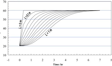
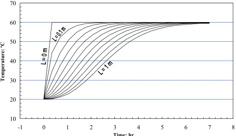
Figure 1. Variation of air temperature in different layers of rock bed.

10

20

30

40

50

60

70

-1

0

1

2

3

4

5

6

7

8

Time: hr

Temperature

: °

C

Figure 2. Variation of rock temperature in different layers of rock bed.

Time: hr

Time: hr

Temperature: ºC

(5)

10

20

30

40

50

60

70

-1

0

1

2

3

4

5

6

7

8

Time: h

Temperature

:

°

Figure 3. Comparison of rock and air temperatures variation.

10

20

30

40

50

60

70

-0.1

0

0.1

0.2

0.3

0.4

0.5

0.6

0.7

0.8

0.9

1

1.1

Length of rock bed: m

Temperature

: °

C

Figure 4. Variation of air temperature along bed with time.

Time: hr

Length of Rock Bed: m

Time = 0 hr

3.5 hr

(6)

10

20

30

40

50

60

-0.1

0

0.1

0.2

0.3

0.4

0.5

0.6

0.7

0.8

0.9

1

1.1

Length of rock bed: m

Temperature

: °

C

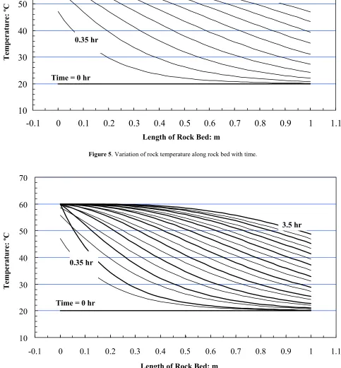
Figure 5. Variation of rock temperature along rock bed with time.

10

20

30

40

50

60

70

-0.1

0

0.1

0.2

0.3

0.4

0.5

0.6

0.7

0.8

0.9

1

1.1

Tempreature

: °

C

Figure 6. Comparison of rock and air temperatures variation along the rock bed length with time.

Length of Rock Bed: m

Time = 0 hr

3.5 hr 3.5 hr

0.35 hr

(7)

10

20

30

40

50

60

70

-1

0

1

2

3

4

5

6

7

8

Time: hr

Temperature

: °

C

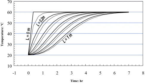
Figure 7. Variation of air temperature in different layers of rock bed.

10

20

30

40

50

60

70

-1

0

1

2

3

4

5

6

7

8

Time: hr

Temperature

: °

C

Figure 8. Variation of temperature in different layers of rock bed.

Time: hr

Time: hr

(8)

10

20

30

40

50

60

-1

0

1

2

3

4

5

6

7

8

Time: hr

Temperature

: °

Figure 9. Comparison of air and rock temperatures variation in different Layers of rock bed.

10

20

30

40

50

60

70

-0.1

0

0.1

0.2

0.3

0.4

0.5

0.6

0.7

0.8

0.9

1

1.1

Length of rock bed:

Temperature

:

°

Figure 10. Variation of air temperature along the rock bed length with time.

Time: hr

Time = 0 hr

3.5 hr

(9)

10

20

30

40

50

60

70

-0.1 0

0.1 0.2 0.3 0.4 0.5 0.6 0.7 0.8 0.9

1

1.1

Length of rock bed

Temperature

:

Figure 11. Variation of rock temperature along the rock length with time.

10

20

30

40

50

60

70

-0.1

0

0.1

0.2

0.3

0.4

0.5

0.6

0.7

0.8

0.9

1

1.1

Temperature

: °

C

Figure 12. Comparison of air and rock temperatures along the rock bed length with time.

Length of Rock Bed: m

Time = 0 hr Time = 0 hr

Time = 0 hr

3.5 hr 3.5 hr

0.35 hr

(10)

In Equation 28, considering x = 2, …, n-1, we will have a set of equations which can be written in form of a matrix. This matrix is solved for variation of air temperature at each location in the rock bed at the end of the time interval _∆t, starting from initial conditions at t = 0 and using Equation 29 and Ta. The variation of rock temperature can also be calculated.

Considering the case where k1, k2 and k3≠ 0 in

Equations 9 and 10, Equation 9 can be written in terms of finite difference as:

-GTa(x-1,t+1)+HTa(x,t+1)+GTa(x+1,t+1)-Ts(x,t+1)

=LTa(x,t)+k1T∞

(30) for (n-1> x > 2)

where

G= 1/2_∆x

H = (1+k1)+(k3/∆t))

M = 1/_∆x L= k3/∆t

N= (1/_∆x + (1+k1)+(k3/∆t)

Equation 10 can also be written in terms of finite difference for (n-1> x > 2):

-CTs(x-1,t+1) + FTs(x,t+1) - C Ts(x+1,t+1)-Ta(x,t+1)

= ETs (x,t)

(31) for x = 1

ATs(x,t+1) + BTs(x+1,t+1) - C Ts(x+2,t+1)-Ta(x,t+1)

= ETs (x,t)

(32) for x = n

A Ts(x, t+1) + BTs(x-1,t+1) - CTs(x-2,t+1) -Ta(x,t+1)

=ETs (x,t)

(33) where

A= ((1/ _∆t ) + 1 –(k2/(∆x)2))

B= 2k2/(∆x)2

C= k2/(∆x)2

E= 1/_∆t

F = ((1/_∆t) +1+ (2k2/(∆t)2)

10

20

30

40

50

60

-0.1

0

0.1

0.2

0.3

0.4

0.5

0.6

0.7

0.8

0.9

1

1.1

Length of rock bed:

Temperature

: °

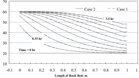
Figure 13. Comparison of rock temperature along the bed length for cases 1 and 2.

Length of Rock Bed: m

Time = 0 hr 0.35 hr

(11)

4. RESULTS

Two cases are considered in this work. In the first case k1 and k2 are considered to be negligible (i.e.

k1 and k2 can be ignored in Equations 9 and 10).

Figures 1 and 2 show the air and rock bed temperature variation with respect to the time respectively. The sets of curves in Figures 1 and 2 differ by the value of Z = βtcoll.. The air

temperature is 60 0_{C at t = 0, as shown in Figure 1.}

This is the condition of air before introducing into the rock bed. The rock bed is divided into n layers and air temperature profile is shown in Figure 1. This figure shows the time required for complete charging of rock bed is 7 hours. The temperature profiles of rock bed layers are shown in Figure 2 at different time intervals. The hot air gives its heat quickly to the rock bed due to high heat transfer coefficient. At the beginning, the temperature of the rock bed gradually increases. Heat is transferred gradually to the other layer. After 7 hours, the temperature of the exiting air begins to rise. This is a sign of charging of the rock bed. Figure 3 compares the air and rock bed temperature profiles. As the time increased, the air and rock bed temperature profiles get closer the each other. Figure 4 shows the air temperature variation along the length of the bed. At t = 0, the air temperature is 60 0C. As is shown in Figure 4, the exit air temperature drops at very short times. As time goes on, the temperature of the exiting air is increased. After 3.5 hours, the exit temperature is about 49 0C. The rock bed temperature variation along the length of the bed is shown in Figure 5. Figure 6 compares variation of air and rock bed along the length of the bed.

In the latter, the coefficients k1, k2 and k3 are

not neglected in the solution. Figures 7 and 8 show the temperature variation of air and rock bed with respect to time. It shows thermal wave dispersion throughout the rock bed. The time rate of change or slope of a curve at particular time shows the impulse response in Figures 7 and 8. Figure (9) compares temperature variation of air and rock bed. As the time increased the temperature profiles of air and rock bed get closer to each other. Figures 10 and 11 show temperature variation of air and rock bed along the bed length. Figure 12 compares the temperature profiles of air and rock bed along

length of the rock bed. As the time increass, the air and rock bed temperature profiles get closer to each other.

5. CONCLUSION

An analytical solution can be written for Equations 5 and 6 with mere boundary condition of T(0,t) = T(1,t) in the inlet air temperature. In this case, the solution is limited to relatively small values of time. In order to extend solution to real case where an initial non-uniform spatial temperature distribution within the bed is considered at large time, initial boundary condition 11 and 12 are to be incorporated in the solution. The solution shows the response of the rock bed during the charging period (energy recovery mode) and the profiles of air and rock bed temperatures with respect to time and length of the bed. Equations 23 and 24 must, therefore, be expressed in finite difference form and solve by numerical procedure. Since the air is used as the heat transfer medium at low temperature, the effect of k1, k2 and k3 (heat loss, conduction through solid

and heat capacity of fluid respectively) are found to be negligible in the solution of the case of air as a moving fluid.

6. NOMENCLATURE

A cross section area of bed, m2 Ca heat capacity of the air, J/kg oC

Cs heat capacity of the rock, J/kg oC

d rock equivalent diameter, m D rock bed diameter m f void fraction %

G air mass flow rate per unit cross section, kg/m2_s

hv volumetric convective heat transfer

coefficient, W/m3 o_C

ks heat conductivity of the rock W/m oC

k1 U/hvD

k2 hvkp/G2Ca

k3 ρaCaf//ρsCs(1-f)

Ta air temperature, oC

Ts rock bed temperature, oC

T_∞ surrounding temperature of rock bed, o_C

(12)

x distance along the rock bed, m

ρa air density, kg/m3 ρs rock density, kg/m3

7. REFERENCES

1. Schmann, T. E. W., “Heat Transfer: A Liquid Flowing Through a Porous Prism”, J. Franklin Institute, Vol. 208, (1929), 405-416.

Rock Bed”, Solar Energy, Vol. 29, No. 6, (1982), 451-462.

4. Cebelli, A., “Storage Tanks-A Numerical Experiment”,

Solar Energy, 19 (1), (1972), 45-54.

5. Duffie, J. A. and Beckman, W. A., “Solar Engineering of Thermal Processes”, 2nd_{Ed., John Wiley and Sons, New}

York, (1980).

6. White, H. C. and Korpela, S. A., “On Calculation of the Temperature Distributions of a Packed Bed for Solar Energy Application”, Solar Energy, 23, (1979), 141-144.

7. Close, D. J., “A Design Approach for Solar Processes”,