Modeling the Time Windows Vehicle Routing Problem in Cross-Docking Strategy Using Two Meta-Heuristic Algorithms

Please cite this article as: M. B. Fakhrzad, A. Sadri Esfahani, Modeling the Time Windows Vehicle Routing Problem in Cross-docking Strategy Using Two Meta-heuristic Algorithms. International Journal of Engineering (IJE) Transactions A: Basics, Vol. 27, No. 7, (2014): 1113-1126

International Journal of Engineering

J o u r n a l H o m e p a g e : w w w . i j e . i r

Modeling the Time Windows Vehicle Routing Problem in Cross-docking Strategy

Using Two Meta-heuristic Algorithms

M. B. Fakhrzada*_{, A. Sadri Esfahani}b

Department of Industrial Engineering, Faculty of Engineering, Yazd University, Yazd, Iran

P A P E R I N F O

Paper history: Received 19 May 2013

Received in revised form 22 October 2013 Accepted in 21 November 2013

Keywords:

Cross-docking Strategy Vehicle Routing Problem Time Windows Tabu Search

Variable Neighborhood Search

A B S T R A C T

In cross docking strategy, arrived products are immediately classified, sorted and organized with respect to their destination. Among all the problems related to this strategy, the vehicle routing problem (VRP) is very important and of special attention in modern technology. This paper addresses the particular type of VRP, called VRPCDTW, considering a time limitation for each customer/retailer. This problem is known as NP-hard problem. Two meta-heuristic algorithms based on the Tabu search (TS) algorithm and variable neighborhood search (VNS) are proposed for its solution. These algorithms are designed for real-world cases and can be generalized to the more complex models such as those which deliveries can be specified in a split form. The proposed TS algorithm also offers a candidate list strategy which has no limitation for the number of nodes and vehicles. A computational experiment is performed to verify our presented algorithms. Through computational experiments, it is indicated that the proposed TS algorithm performs better than VNS algorithm in both aspects of the total cost and computation time.

doi:10.5829/idosi.ije.2014.27.07a.13

1. INTRODUCTION1

Over the recent years, many companies confronted with more complicated and various customer demands. Thus, many companies are trying to achieve high level of agility, flexibility and reliability for various demands [1]. In the real world, the production procedure consists of purchasing raw material from suppliers, producing or manufacturing, storing and delivering the final product to customers. These systems that start by suppliers and end by customers are called supply chain systems [2]. In such systems, operations of a single company necessarily make no improvement in customer’s satisfaction, because its operations may have interacting effects or even adverse effects on other companies in the supply chain system [1]. For this reason, nowadays, supply chain management is one of the most attractive issues in operational management. Apte and Viswanathan [3] express that over 30% of goods price is incurred in distribution process. Thus, the efficient

*Corresponding Author Email: [email protected] (M. B. Fakhrzad)

1. 1. Cross-docking Apte and Viswanathan [7] introduced cross-docking as one of the most strategic and technologic innovations in the supply chain management. In this system, cross docks/distribution centers function as inventory coordination points rather than as inventory storage points [6]. In the cross-docking, all deliverable products arrive to the cross dock and are immediately categorized, sorted and organized according to their destinations and customers' demand. Then, these products are moved to respective destinations, without storing in the cross dock. In other words, in the cross-docking systems, a few stocks are handled in temporary storage [8]. In this strategy, products usually are stored less than 12 hours at the cross dock ([3, 9]), sometime less than an hour [10]. Figure 1 illustrates the flow of material in the cross docking.

Cross-docking includes two key processes that are depicted in Figure 1. The pickup process is the product/material flow from supplier to the cross dock and the delivery process is the product/material flow from cross dock to customer. The key issues in the pickup and delivery processes are the simultaneous arrival at the cross dock and consolidation, respectively. The purpose of consolidation is to categorize and to sort the products at the cross dock with respect to their destinations. Regarding to the consolidation process, some of vehicles have to unload their entire burden completely and reload another product(s). Also, some of the vehicles have to unload partial of their products and reload another product(s) and some of the vehicles which have extra capacity, are only loaded with the new product(s). The purpose of simultaneous arrival to the cross dock is to reduce the waiting time of vehicles. If vehicles of the pickup fleet could not arrive at the cross-dock simultaneously, then the consolidation process has been postponed. Thereby, it might increase the waiting time and the inventory level at the cross dock [2].

1. 2. Literature Review and Research Motivation Recently, many studies treated various issues of cross-docking from different viewpoints. These investigations can be divided into two categories: studies that focus on (1) physical aspects of cross docking and (2) operational aspects of cross-docking.

Most of the first-category studies describe the cross-docking concept and its advantages [11-13], physical design of cross dock in cross-docking [3, 14-18], and optimal location of cross dock [19-21]. On the other hand, most of the investigations related to the second-category focused on the trucks scheduling in cross-docking system [8, 22-31]. In addition, over the last 30 years or so, the classical VRP has attended strongly in the literature. The classical VRP involves the service of a set of customers with known demands by a fleet of vehicles from a single distribution center [2].

Figure 1. The concept of cross-docking [1].

The main objective of the problem is to design a set of routes starting and ending at the distribution center/depot such that all customers are serviced and the total cost of the set of routes is minimized [32]. Some of the most recent VRP papers, such as those have been published by Lin et al. [33], Cheng and Wang [34], Catay [32], Mirabi et al. [35] and Zachariadis and Kiranoudis [36]. Mosheiov [37] considered the pickup and delivery problems as a VRP problem and proposed the two heuristic algorithms to find a good solution to minimize transportation cost and maximize the efficiency of vehicles. VRP with time windows (VRPTW) can be very helpful encountering with cross-docking problems [1], because one the core issue in such problems is the simultaneous arrival at the cross dock. In general, time window models can be divided to three categories:

VRP with hard time window (VRPHTW): In such models, vehicles have to service customers in the specific time interval and any violation from the service time window HWV is not admissible for customer

i

, whatsoever.

VRP with soft time window (VRPSTW): In such models, vehicles are allowed to service customers before and after the earliest and latest time window bounds, respectively. If any violation occurs from the service time window[a_i,b_i], by introducing appropriate penalties, measure of customer’s non-satisfaction is reflected [38].

VRP with hard and soft time window (VRPHSTW): Such models are combination of the two mentioned models. Time window in these models include a hard and a soft interval. Hard interval cannot be violated and soft interval can be violated [38].

supply chain management by minimizing total transportation cost. Hasani-Goodarzi and Tavakkoli-Moghaddam [40] considered a split vehicle routing problem (SVRP) with capacity constraint for multi-product cross-docks. Mousavi and Tavakkoli-Moghaddam [41] presented a two-stage mixed-integer programming (MIP) model for the location of cross-docking centers and vehicle routing scheduling problems with multiple cross-docking centers due to potential applications in the distribution networks. To the best of our knowledge, there have been a few papers that take both cross-docking and time scheduling with time windows into consideration simultaneously. Ma et al. [42] proposed a new shipment consolidation and transportation problem in cross-docking distribution networks by considering setup cost and time window constraint. Ma et al. [42] considered direct rout to-retailer) as well as indirect rout (supplier-to-cross dock and cross dock-to-retailer). Ma et al. [42] also assumed that products can be stored at the cross-dock for relatively long times. Dondo and Cerdá [43] introduced a sweep heuristic for the VRPCD that determines pickup/delivery routes and schedules simultaneously with the truck scheduling at the terminal. Dondo and Cerdá [43] assumed that the pickup/delivery nodes should be visited within specific hard time windows. Unlike Ma et al. [42] and Dondo and Cerdá [43], this paper considers the multi-commodity consolidation and soft time windows for each delivery node. In this paper, it is assumed that all deliverable products are moved to respective destination without storing in the cross-dock. It is also assumed that direct shipping from the suppliers to retailers is not allowed. In this paper, the primary motivation is to present two algorithms for the solution of the above-described complex model of cross docking strategy.

This paper is organized as follows: section 2 presents the model assumptions and formulation. Section 3 describes the tabu search and variable neighborhood search algorithms for VRPCDTW and presents the steps of the algorithms. Section 4 compares the performance of the proposed algorithm. Finally, section 5 concludes the paper and presents the future research.

2.MODELASSUMPTIONSANDFORMULATION

The problem considered in this study, namely VRPCDTW, is VRP cross-docking with time window. The problem formulation is based on the following assumptions:

· This problem is goods transportation from a set of suppliers to a set of corresponding customers/retailers through a cross-dock. Direct shipping from the suppliers to retailers is not allowed.

· A soft time window is considered for each customer.

· A set of identical vehicles is used to transport goods from supplies to retailers.

· Consolidation process must be accomplished at the cross dock.

· The whole process must be completed in the planning horizon.

· Each supplier or retailer can only picked up or delivered once. Each location (pick up/delivery node) cannot be visited by the same vehicle more than once.

· No intermediate storage in the cross-dock is allowed.

· There are no pre-defined vehicles for some suppliers and retailers.

The main objectives are to determine the number of vehicles and the best routes and schedules to minimize the sum of transportation cost, vehicle operation cost and time window violation cost. The notations (sets, parameters and decision variables) and mathematical formulation are as follows. It should be noted that some of the used notations in the proposed model, are similar to that of Wen et al. [10]:

P

: set of nodes in the pickup process D: set of nodes in the delivery process

0

: cross dock index

n

: number of suppliers/retailers NV: number of available vehicles

Q: capacity of the vehicle(pallet)

A

: the fixed time for loading, unloading and reloading at the cross-dock and each node

B

: the time for loading, unloading and reloading a pallet at the cross-dock and each node

ij

tc

: transportation cost from node ito node

j

n

o

: operation cost of vehicle

n

. It should be noted that all of the vehicles have an identical operation cost.

ij

t

: travel time between node

i

and

j

i

p

: number of pallets loading in pickup node

i

i

d

: number of pallets unloading in delivery node

i

n i

DT : departure time of vehicle

n

from node

i

n

AT

: arrival time of vehicle

n

at the cross dock

n i

S : service start time of vehicle

n

at node

i

i

yen : amount of start time earliness of vehicle

n

at node

i

i

yl

_n : amount of start time lateness of vehicle

n

at node

i

e

P: unit penalty cost for earliness

l

i

e

: lower bound of hard time window at node

i

i

l

: upper bound of hard time window at node

i

i

LB: lower bound of soft time window at node

i

i

UB: upper bound of soft time window at node

i

M : very big number

T

: time horizon

Decision variables:

n

ij

x

: if the vehicle

n

move from the node

i

to the node

j

, 1, otherwise,0. (

i

,

j

Î

P

or

D

)

n

i

u

: if the vehicle

n

unload the goods

i

at the cross dock,1, otherwise,0. (

i

Î

P

)

n

i

r

: if the vehicle

n

load the goods

i

at the cross dock,1, otherwise,0. (

i

Î

P

)

n

tu

: the time at which vehicle

n

finishes unloading at the cross dock

n

tr

: the time at which vehicle

n

starts reloading at the cross dock

i

v

: the time at which goods

i

is unloaded at the cross dock

Mathematical model:

0

1 1 1 1 1

1 1

2 ( . . ) n n NV NV n

ij ij j

i j j

n NV

e i l i i

i D

Min tc x o x

P ye P yl

n n n n n n n n = = = = = = = Î + + +

ååå

åå

åå

(1) . .

t

s

j x n i NV

ij = "

åå

= =

, 1 1n 1

n (2) i x n j NV ij = "

åå

= = , 1

1n1

n

(3)

n

n _{£ "}

å

= , 1 1 0 n j j x (4) n

n _{£ "}

å

= , 1 1 0 n i i x (5) n n

n _{0, ,}

1 1 p x x n j pj n i

ip-

å

= "

å

=

= (6)

n

n

n _{£ "}

åå

= = NV n j j NV x 1 1

0 , (7)

n

n _{£ "}

å

Î = , ,1 Q x p ij n P j i

i i (8)

n

n _{£ "}

å

Î = , ,1 Q x d _ij n D j i i i ₍₉₎ ( . ). , ,

j ij i i ij

DTn ₌ t ₊DTn ₊A₊p B xn _"n j_ÎP ₍₁₀₎

( . ). , ,

j ij i i ij

DTn ₌ t ₊DTn _{+ +}A d B xn _"n j_ÎD ₍₁₁₎

å

å

Î= Î= = n D i i i n P i i i d p 1 1 (12)

1 1 1 1

1 1 1 1

( . ). ( . ).

. . ,

n n n n

i ij i ij

i j i j

i P j P i D j D

n n n n

ij ij ij ij

i j i j

i P j P i D j D

A p B x A d B x

t x t x T

n n

n n _n

= = = =

Î Î Î Î

= = = =

Î Î Î Î

+ + + +

+ £ "

å å

å å

å å

å å

(13)

P i x t DT

AT =( i + i0). i0,"n, Î n n n ₍₁₄₎ n n n

n _=AT ¢_{," ¹ ¢}

AT (15) j i t DT x M

Sn_{j +} (1_- n_ij)_{- i}n _{- ij³}0,_"n, , ₍₁₆₎

D i UB S

LBi£ in£ i,"n, Î (17)

D i S e

yen_i³ _i- _in, Î (18)

D i l S

yli³ i - i,"n, Î

n

n (19)

P i r

uin+ in£1,"n, Î (20)

P i x x r u D j j n i P j ij i

i - =

å

-

å

" Î

È Î + È Î , , 0 , 0 n n n n n ₍₂₁₎ n n n _{³tu ,"}

tr (22)

P i u M

tu ³ni- (1- i),"n, Î n n (23) P i r M

trn ³ni- (1- in),"n, Î (24)

{ }

i j PorD r

u

xijn, in, inÎ 0,1,"n, , Î (25)

0 ,

,tr _i³

tun n n ₍₂₆₎

The objective function of this problem is expressed by Equation (1). It is tried to minimize the sum of transportation cost, operation cost of vehicles and, earliness and lateness of vehicles cost. Equations (2) and (3) show that one vehicle has to arrive at and leave one node. Equations (4) and (5) show that one vehicle has to leave the cross dock from one node and arrive at one node at the cross dock. Equation (6) expresses the consecutive movement of vehicles. Equation (7) shows that the number of vehicles that leave the cross-dock must be less than the number of available vehicles,NV. Equations (8) and (9) express that the quantity of loaded products in a certain vehicle cannot exceed the maximum capacity of the vehicle in the pickup and delivery processes, respectively. Equations (10) and (11) express that the departure time of a vehicle from node,j, is determined by the sum of the departure time

Equilibrium equation is shown in Equation (12). In Equation (13), the sum of the total length of the visit to each node and total transportation time must be less than the planning horizon, T. The arrival time at a cross-dock is represented by Equation (14). The constraint for simultaneous arrival to a cross-dock is given in Equation (15). Equation (16) determines the service start time for each node. The constraint for soft time windows is represented in Equation (17). Equations (18) and (19) determine the amount of earliness and lateness of a start time. This fact that a vehicle,

n

should unload or reload product, i, depends on its pickup and delivery routes is expressed by Equation (20). Equation (21) shows the linkage between the pickup and delivery process in the consolidation decisions at the cross dock. Equation (22) indicates that a vehicle cannot start reloading until it finishes unloading. Equations (23) and (24) express the time at which vehicle,

n

finishes unloading and starts reloading at a cross dock.

3.META-HEURISTICSFORTHEVRPCDTW

SinceVRPCDTW is considered as a NP-hard problem [1], an efficient meta-heuristic method is needed to achieve a good solution in a reasonable amount of time. TS was successfully applied to solve the various types of VRP [1, 2, 44, 45]. VNS was also successfully applied to solve the multi depot routing problem [46] and scheduling the trucks in cross-docking systems [26]. In this paper, two meta-heuristics algorithms based on TS and VNS are presented to solve the VRPCDTW. Sections 3.1 and 3.2 are devoted to the TS-based and VNS-based algorithms, respectively.

3. 1. A TS-based Meta-heuristic for the VRPCDTW

TS is an iterative local search algorithm, which cycling back to previously visited solution is prevented by the use of memories. TS was originally developed by Glover [47]. Some of the basic components of TS method are: initial solution, neighborhood structure, stopping criteria, tabu list and aspiration criteria. TS, at each iteration, explores the solution space and tries to make the best possible moves from the current solution

x

to the best solution

x

¢

in its neighborhood N(x), even if the move may deteriorate the objective function value. A tabu mechanism is put in place to prevent the process from cycling over a sequence of solutions. TS exploits tabu list to prevent cycling and local optima. Some attributes of the past solutions are registered and any solution possessing these attributes may not be considered. Temporarily are also declared tabu forq iterations (it is called tabu tenure). However, tabu moves can be overridden if the aspiration criterion is

satisfied. Here, a TS-based heuristic to solve the VRPCDTW is developed.

3. 1. 1. Initial Solution Similar to the other local search algorithms, TS is an iterative procedure that starts from an initial solution. This solution is the starting point for subsequence exploration in the solution space. Here, an initial solution scheme for VRPCDTW is introduced.

Pickup process:

1) Calculate the minimum number of vehicles.

å

= p Q

NVmin _i/

2) Sequence vehicles in descending order of the remaining space. In the stage of initialization, all of the vehicles are available at the cross dock. They are empty and sort according to their index.

min

,..., , 2 1 S SNV S

3) Determine all possible routes that the first vehicle can be moved in the sequence of step 2. Calculate the ratio of transportation cost to the minimum transportation cost between the determined routes. Generate the candidate list of routes that their calculated ratios are less than

a

. Select a route and its related node randomly from the candidate list.

4) Replicate the steps 2 and 3 until all nodes are assigned. If the remaining capacity of a vehicle is less than the supply of node

i

, select next vehicle in the sequence of step 2. If no vehicle was found, add one additional vehicle to the set of vehicles.

Delivery process

1) Calculate the remaining time for delivery process,. td=T-tp where,

t

_d is the remaining time for delivery

process,

T

is the time horizon and

t

_p is the completion time of the pickup process.

2) All vehicles travel to the corresponding customer without any consolidation. For example, if the first vehicle is made pickups in the nodes 1, 2 and 4, thus, shipment of this vehicle must be delivered to the customers 1, 2 and 4.

3. 1. 2. Objective Function Evaluation The proposed TS algorithm is based on that of Cordeau et al. [48], in which the infeasible solutions are allowed during the search.

( ) ( ) ( )

( ) . ( )

f s c s TV s

HWV s M SWV s

a b

= + +

+ (27)

where, f(s) is the objective function in the algorithm iterations,

c

(s

)

is the original objective function defined in (1), TV, HWVandSWVare the violation measures for delivery process remaining time, hard time windows and soft time windows, respectively. If the solution is feasible for these three constraints, TV,

HWVand SWVare equal to 0.

a

and

b

are the penalty coefficients for the time horizon and hard time windows violation, respectively. In order to satisfy the soft time windows, a big penalty coefficient (

M

) is considered for SWV. TV_, HWV_and, SWVare defined as follows:

) ). (

(

0 0 1

d j

j NV

D j

j A d B t x t

S

TV=

å å

+ + + _j

-= Î

n n

n

(28)

1

1

[ [ (( . ). ) ]]

[ [ ( . ) ]]

NV

i i ij i

i D j D NV

i i ij i D j D

HWV S A d B x l

e S x

n n

n

n n n

+

= Î Î

+

= Î Î

= + + - +

-å -å -å

å å å

(29)

1

1

[ [ (( . ). ) ]]

[ [ ( . ) ]]

NV

i i ij i

i D j D NV

i i ij i D j D

SWV S A d B x UB

LB S x

n n

n

n n n

+

= Î Î

+

= Î Î

= + + - +

-å -å -å

å å å

(30)

where(x)+=max(0,x)_.

It should be noted that the initial solution is designed in such a manner that the vehicles capacity have no violation. However, during the search algorithm, vehicle capacity may be violated. Therefore, a penalty coefficient for the capacity violation measure is considered. According to the above discussion, f(s)is modified as follows:

( ) ( ) ( ) ( ) . ( ) ( )

f s c s TV s HWV s

M SWV s CV s

a b

g

= + + +

+ (31)

where, CVand

g

are the capacity violation measure and

its penalty coefficient, respectively.

3. 1. 3. Neighborhood Structure Neighborhood structure is the transformation mechanism that applies on the current solution to generate candidate solution. Insertion and exchange are the most simple and famous mechanisms to generate neighboring solution in the heuristic algorithms. Recently, _2-opt* _{and CROSS}

mechanisms have generated good solutions. In the insertion mechanism, one node

i

removes from its original vehicle

k

and re-inserts to another vehicle

k

¢

. However, in the exchange mechanism, two nodes belonging to the two vehicles are swapped. 2-opt operator is applied in this paper. One vehicle is selected

randomly and then two routes whose transportation cost between two nodes is more than the other nodes are found. These two selected routes are exchanged with the two corresponding routes in another randomly selected vehicle. If there are not any corresponding routes in the two randomly selected vehicles, then, the sequence of the two routes is changed in the first selected vehicle.

3. 1. 4. Candidate List Strategy For a given solution,

x

, it is computationally too expensive to explore its whole neighborhoods. Thus, in the proposed algorithm, instead of examining all neighborhoods,N(x)

, a candidate list consisting of vehicles which have the most number of nodes is examined. For example, if the number of vehicles is more than a certain number (i.e. 5 vehicles), the known percent of vehicles (i.e. 50%) which have the most number of nodes are examined.

3. 1. 5. Tabu Status and Tabu List One of the TS’s objectives is to encourage the exploration of parts of the solution space that have not been visited previously [45]. The complete solutions are not kept in the tabu list. The attributive memory is used for the tabu list, and the e-attributes of an accepted move are stored [49]. For 2-opt operator, the tabu status of the solution is defined by the vertex pair (i, j). These two vertices are stored in the tabu list, and any solution possessing these attributes may not be considered and temporarily declare the tabu for

q

iterations. In this paper, two tabu lists are defined for both pickup and delivery processes. Each tabu list is an

n

´

n

matrix, where element TABU _j(i,k) specifies the tabu status of

arc (i,k) in TABU_j. If TABUj(i,k)£0, arc (i,k) is not a

tabu; otherwise tabu.

3. 1. 6. Aspiration Criterion In the TS algorithm, tabus may prohibit attractive moves, even when there is no danger of cycling. Hence, it is necessary to use algorithmic devices to allow one to revoke tabus. These are called aspiration criterion. In this paper, similar to the almost all of the TS implementation, most commonly aspiration criterion is used. In this aspiration criterion, a tabu move can be overridden if it has less objective value than the best solution found so far.

3. 1. 7. Stopping Criterion In this paper, when the maximum iteration bound determined by the user is reached, the search is stopped. The iteration number is calculated by the following formula:

) 1 1 (

F NV

E´ + - (32)

3. 1. 8. Proposed Algorithm Steps Before describing the algorithm flow and presenting the flowchart of the algorithm, some parameters are introduced in the following:

P

c

n

: current number of the generated candidate solutions, in the pickup side;

D

c

n

: current number of the generated candidate solutions, in the delivery side;

max

n : maximum number of the candidate moves;

P

A

: set of candidate solutions in the pickup process;

D

A

: set of candidate solutions in the delivery process; count: counter of iterations;

NUI: current number of iterations without

improvement;

max

iteration : maximum number of algorithm iterations;

max

NUI : maximum number of iterations allowed without improvement;

*

x

: the best-found solution;

h

: adjusting coefficient for the penalty coefficients;

Step 1 Initialization

1.1) Generate an initial solution (

x

) based on 3.1.1.

1.2) Set the algorithm parameters,

a

,

b

,

g

,

h

,

max

NUI , tabu tenure(

q

),

TABU

(

i

,

k

)

=

f

,

E

,F,

1

=

count , and NUI=0. Calculateiteration_max based on (32).

1.3) set:

x

*

¬

x

_and

f

(

x

*

)

¬

f

(

x

)

_.

Step 2 Generate the admissible solution in the pickup side

Set ₌₁

P

c

n andAP =f.

2.1) If

max n

n_cP ³ , go to step 3.

2.2) Based on section 3.1.4, determine the vehicle candidate list for generating the neighborhoods. Apply predetermined neighbor-generating method described in section 3.3. A solution

P c n

x is generated from the

neighborhood N(x)of

x

and added to the candidate solution. Set,

P c

n P P A x

A ¬ È , _{¬ +1}

P

P c

c n

n and go to

step 2.

Step 3 Select the best move in the pickup side

amongst A_P

Evaluate all the solutions in

A

_Paccording to section 3.2. Put all non-tabu solution inN¢(x), seti=1,

initial

best

x

x

P

=

,

f

(

x

bestP

)

=

f

(

x

initial

)

. Put all tabu

solutions inN¢¢(x).

3.1) Ifi>n_max, go to step 4.

3.2) If xiÎN¢(x)UN¢¢(x) and f(xi)£ f(xbestP),

set: x_bestP¬x_i, i¬i+1and go to step 3.1.

Step 4 Generate the admissible solution in the delivery side

Set ₌₁

D c

n andAD =f.

4.1) If

n

n

_max

D

c

³

, go to step 5.

4.2) Based on section 3.1.4, determine the vehicle candidate list from the solution obtained in step 3, for generating the neighborhoods. Apply exchange operator according to section 3.3. A solution

D c n

x is generated

from the neighborhood N(x)of

x

and added to the

candidate solution. Set:

D c n D D A x

A ¬ È ,

1 +

¬ _D

D c

c

n

n

and go to step 4.1.

Step 5 Select the best move in the delivery side

amongst A_D

Evaluate all solutions in A_Daccording to section 3.1.2. Put all non-tabu solution inN¢(x), seti=1,

P best best

x

x

=

,

(

)

(

)

P

best

best

f

x

x

f

=

. Put all tabu

solutions inN¢¢(x).

5.1) Ifi>n_max, go to step 6.

5.2) If x_iÎN¢(x)UN¢¢(x) and f(x_i)£ f(x_best ), set:

i

best

x

x

¬

. i¬i+1and go to step 5.1.

Step 6 Update the statistical information

If f(x_i)³ f(x_best ), set NUI¬NUI+1and go to

step 1. Otherwise: set

x

*¬

x

_{best and}

) ( ) ( *

best x f x

f ¬ .

Step 7 Update the memory structure

Update the tabu list according to

x

*_{. Set}

1 ) , ( )

,

(ik ¬TABU i k +

TABU_j , j=1,2 where the indices

1 and 2 demonstrate the pickup and delivery processes, respectively.

Step 8 Update the penalty coefficients

If the current solution is feasible with respect to each items of the objective functions (TV,HWV ,SWV and CV), the value of the corresponding penalty coefficient is divided by

1

+

h

; otherwise, it is multiplied by1+h.

Set count¬count+1.

Step 9 Stopping

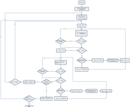
The flowchart of the proposed algorithm is given in Figure 2. In addition, the pseudo code of the TS algorithm is given below.

1. Begin

2. Generate an initial solution.

3. Set the initial solution as the current and also the best solution.

4. Generate an empty list for keeping the frequency of the solution changes in the pickup side.

5. Generate an empty list for keeping the frequency of the solution changes in the delivery side.

6. While stopping criterion is not met do

7. For nc_p=1to nmax=1

Search the neighborhood of the current solution in the pickup side.

current solution¬neighborhood of thecurrent solution . Then update the tabu list.

8. If

current solutionobjective function bestsolutionobjective function< then

9. best solution¬current solution

10. _Endif

11. Endfor

12. current solution¬best solution

13. For n_cd=1to nmax=1

Search the neighborhood of the current solution in the delivery side.

current solution¬neighborhood of thecurrent solution _.

Then, update the tabu list.

14. If

current solutionobjective function best solutionobjective function<

best solution¬current solution

15._Endif

16.Endfor

17.Endwhile

18.End

3. 2. A VNS-Based Meta-heuristic for the VRPCDTW VNS is a new meta-heuristic for solving the combinatorial and global optimization problems that proposes systematic changes of the neighborhood structure during the search. VNS originally proposed by Hansen and Mladenovic [50]. Basic idea of the VNS is a systematic changing of neighborhood both within a descent phase to find a local optimum and within a perturbation phase to get out of the corresponding valley [51]. VNS explores close and then increasingly far neighborhoods of the best known

solution in a probabilistic way. In other word, VNS applies a local search procedure repeatedly to get from neighboring solutions to local optima [51]. Because of relying on very few parameters, such as stopping criterion and number of neighborhoods, VNS is very easy to implement. A very comprehensive study about VNS can be found in Hansen and Mladenovic [50, 52]. Here, a VNS-based heuristic to solve the VRPCDTW is developed.

3. 2. 1. Initial Solution Similar to the other meta-heuristic algorithm, an initial feasible solution is necessary to start VNS procedure. In this paper, initial solution scheme described in TS algorithm is applied, as initial solution.

3. 2. 2. Neighborhood Structures In almost all of the meta-heuristic algorithms, one or more neighborhood structures is utilized as a means of defining admissible moves to transition from one solution to another solution. Because of the good performance, 2-opt operator is applied in this paper. One vehicle is randomly selected and then two routes whose transportation cost between two nodes is more than the other nodes are found. These two selected routes are exchanged with the two corresponding routes in another randomly selected vehicle. If there are not any corresponding routes in the two randomly selected vehicles, then, the sequence of the two routes is changed in the first selected vehicle.

3. 2. 3. Shake Procedure The shake procedure generates a x¢at random from neighborhood of

x

, i.e.

( )

x¢ÎN x .

3. 2. 4. Stopping Criterion In this paper, the stopping criterion is determined by the maximum number of iterations between two improvements. In this paper, the iteration number is calculated by formula (32).

3. 2. 5. Proposed Algorithm Procedure

Step 1 Initialization

1.1) Generate an initial solution (x ) based on 3.1.1.

1.2) Determine the neighborhood structure. In this paper,N_2-opt(.).

1.3) Set the algorithm parameters,

a

,

b

,

g

,

E

,

F

,

1

=

count

. Calculate

iteration

_max based on formula (32).

initia l

x x*¬

1

=

P

c

n

P c n x

P

c n

x

m ax n ncP>

P

c n

x xbestP¬xncP ncP=ncP+1

P P nc best pr evx

x ¬

1

=

D

c

n

D

c n

x

D

c n

x

D c n

x

max n ncD>

D

c n

best x

x ¬ _{= +1}

D D c

c n

n

prevx xbestP¬

1

+ =NUI NUI

max

NUI NUI>

1 + =count count

m ax itera tion count>

Figure 2. Flowchart of the proposed algorithm.

Step 2 shake and local search in pickup and delivery sides

2.1) Shake routine in the pickup side. Find a random solutionx¢ÎN₂-opt( )x .

2.2) Local search in the pickup side. Apply neighborhood structure onx¢ to find a solutionx_pickup. 2.3) Shake routine in the delivery side. Find a random solutionx¢¢ÎN₂-opt( )x .

2.4) Local search in the delivery side. Apply neighborhood structure onx¢¢ to find a solutionx_delivery. 2.5) If_f(_x ) _f(_x*)

pickup < then *

pickup x ¬x . If

) ( ) (_{x f x}*

f delivery < then

*

delivery

x ¬x .

Set: count¬count+1.

Step 3 stopping

If count<iteration_maxthen _{x ¬x}* _{and go to 2.1,} else show_x*_.

The pseudo code of the VNS algorithm is as follows:

1. Begin

2. Generate an initial solution (x ).

3. Set the initial solution as the best solution (x*).

4. While stopping criterion is not met do

5. Repeat the following steps

6. _x¬x*

7. Shake routine in the pickup side. Find a random solutionx¢ÎN₂-opt( )x .

8. Local search in the pickup side. Apply neighborhood structure onx¢ to find a solutionx_pickup.

9. Shake routine in the delivery side. Find a random solutionx¢¢ÎN_2-opt( )x .

10.Local search in the delivery side. Apply

neighborhood structure on

x

¢¢

to find a solutionx_delivery. 11.If _f(_x ) _f(_x*)

pickup < then

12. *

pickup

x ¬x

13.Break

15. *

delivery

x ¬x

16.Break

17.Endif

18.Endif

19.Endwhile

End

4. COMPUTATIONAL EXPREMENTS

The aim of this section is to compare the performance of the two proposed algorithms described in section 3. It should be noted that, to verify and validate the mathematical model, several small size test problems were solved by the Lingo 8 software and optimal results were obtained. Optimal results of the four instances are presented in Table 2.

To evaluate the performance of the proposed algorithms, a computational study is carried out. For this purpose, the proposed algorithms are coded by using Visual Basic programming language. In the implemented programs, route of each vehicle is determined as well as respective costs, such as transportation cost, operation cost and earliness and lateness cost. The performances of the proposed algorithms are verified by comparing the obtained results from TS and VNS with the lower bound solution. The lower bound solution is developed by relaxing the constraints (17)-(19) that related to the time windows. To have a fair comparison both algorithms were executed on a special laptop. Due to lack of benchmark problems in the literature, randomly generated problems are considered. The approach of this paper to randomly design of the time windows is similar to Xiangyong et al. [45] approach as follows: The hard time window is determined by randomly generated and time width , ie., [ , ]= _{− , +} . is an integer randomly generated from interval _{[0 +}

, − −( + )] for each node ∈ , where = .Time width is an integer uniformly

generated from the range [10, 30]. The soft time window is specified by [ , ]= − , +

. Following Lee et al. [1] other parameter values are as follows: capacity of the vehicle (pallet) Q=70,

travel time between node

i

and

j

,

(20,200)

ij

t ºuniform , transportation cost from node i to node j _, tc_ij ºuniform(48,480), number of pallets loading in pickup node

i

and number of pallets unloading in delivery node

i

, p di, i ºuniform(5,50). Also, operation cost of vehicle

n

,

o

_n,unit penalty cost for earliness ,

P

_e, unit penalty cost for lateness ,P_l, the fixed time for loading, unloading and reloading at the cross-dock and each node ,A, and the time for loading, unloading and reloading a pallet at the cross-dock and each node ,B, are specified by 100, 5, 5, 10 min and 1

min, respectively. In this paper, the approach of the parameters setting is similar to response surface methodology (RSM). For this purpose, critical factors of the TS algorithm that are statistically significant in aspects of performance and CPU time have been identified. Critical factors of the TS algorithm based on Vahdani and Zandieh [26] are maximum iteration (

max

iteration ), maximum number of iterations allowed without improvement (NUI_max), maximum number of

the candidate moves (n_max) and tabu tenure (q).

According to the determined neighborhood structure, the critical factor of the VNS algorithm isiteration_max. By preliminary experiments, parameters of the proposed algorithms have been tuned, with which the algorithm had a relatively better performance and CPU time. Parameter setting is presented in Table 1.

Total cost comparison results of the two proposed algorithms versus Lingo results for the sample instances are provided in Table 2. The time horizon T is supposed to be 600 min.

Comparison results show that while using the Lingo software, the solution time is exponentially increased by increasing the number of nodes, whereas the proposed algorithms can solve the problem in much less time. Table 2 also shows that the presented algorithms can generate near optimal solution for the sample problems. Therefore, these algorithms can efficiently solve large size problems in the logical time. Comparative results of total costs and computation times of the TS and VNS algorithms as well as the lower bound solution for randomly generated large size instances are provided in Table 3 and Table 4, respectively. It should be noted that the value of each instance was reported from the average of 10 repetitions. Percentage gap between the total costs of the two presented algorithms and lower bound solution is calculated according to the following formula (I).

cos cos

cos 100

tota l t of the proposed a lgor ithm tota l t of the lower bound solution tota l t of the lower bound solution

Ga p = - ´ (I)

TABLE 1. Parameter setting

Parameter Definition Value for TS Value for VNS

a

penalty coefficients for the time horizon violation 100 100

b penalty coefficients for hard time windows violation 100 100

g

penalty coefficient for capacity violation 50 50

h

adjusting coefficient for penalty coefficients 2 -

E parameter for _iterationmaxbased on formula (32) 60 80

F parameter for _iterationmaxbased on formula (32) 3 2

max

NUI maximum number of iterations allowed without improvement 3n -

max

n maximum number of the candidate moves 50 -

q tabu tenure iterationmax_{2 -}

TABLE 2. Total cost comparison results of the proposed algorithms versus Lingo

Problem No. of available vehicles No. of nodes in each sides (pickup and delivery)

TS result VNS result Lingo

Total cost

cpu time (s)

Total cost

cpu

time (s) Total cost cpu time (s)

VRPCDTW 1 5 5 2583.3 45 2590 48 2501 32

VRPCDTW 2 5 6 2936.75 61 3020 60 2899 48

VRPCDTW 3 5 7 3145.86 65 3266.9 69 3046.32 1180

VRPCDTW 4 5 8 4257.9 150 4320 151 3998.38 26000

TABLE 3. Total cost obtained by TS algorithm for the large size problems (T=600 min)

Problem No. of available _vehicles No. of nodes in each sides _{(pickup and delivery)} Lower bound solution TS result Gap (%) Total cost Total cost cpu time (s)

VRPCDTW5 10 15 7277 8364 100 14.94

VRPCDTW 6 10 20 8834 10036 210 13.61

VRPCDTW 7 20 25 12035 13299 275 10.50

VRPCDTW 8 20 30 12480 14437 486 15.68

VRPCDTW 9 30 40 15980 18907 840 18.32

VRPCDTW 10 30 50 19750 25003 1022 26.60

VRPCDTW 11 50 60 36551 40167 2306 9.89

VRPCDTW 12 50 70 49383 60225 3126 21.95

VRPCDTW 13 60 80 65511 78930 3840 20.48

VRPCDTW 14 60 90 89127 100128 4209 12.34

Average gap (%) 16.43

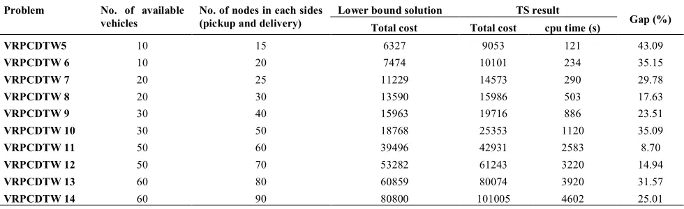
TABLE 4. Total cost obtained by VNS algorithm for the large size problems (T=600 min) Problem No. of available

vehicles

No. of nodes in each sides (pickup and delivery)

Lower bound solution TS result

Gap (%) Total cost Total cost cpu time (s)

VRPCDTW5 10 15 6327 9053 121 43.09

VRPCDTW 6 10 20 7474 10101 234 35.15

VRPCDTW 7 20 25 11229 14573 290 29.78

VRPCDTW 8 20 30 13590 15986 503 17.63

VRPCDTW 9 30 40 15963 19716 886 23.51

VRPCDTW 10 30 50 18768 25353 1120 35.09

VRPCDTW 11 50 60 39496 42931 2583 8.70

VRPCDTW 12 50 70 53282 61243 3220 14.94

VRPCDTW 13 60 80 60859 80074 3920 31.57

VRPCDTW 14 60 90 80800 101005 4602 25.01

As depicted in Table 3, the average gap between the total costs of the TS solution and lower bound solution is 16.43% that is desirable. In addition, Table 4 shows that the average gap between the total costs of the VNS solution and lower bound solution is 26.45%. As a result, computational experiments indicate that the proposed TS algorithm performs better than VNS algorithm in aspect of the total cost.

5.CONCLUSIONANDFUTURERESEARCH

This paper presented a new model, namely VRPCDTW, integrating cross-docking with VRPTW. Since this problem is categorized as a NP-hard problem, two meta-heuristic algorithms based on the TS and VNS were proposed for its solution. The proposed algorithms were shown to have the adequate flexibility while

encountering with the real-world cases. A

computational experiment was carried out to compare the performance of the proposed algorithms. Experimental results showed that the proposed algorithms were capable of solving the large size problems in the logical time. Because of presenting a candidate list strategy, computational experiments indicated that the proposed TS algorithm performs better than VNS algorithm in both aspects of the total cost and computation time. Future research can be suggested in a few directions. It is interesting to solve the proposed model by new meta-heuristic algorithms and compare their results with the results of the proposed algorithms. Another extension is to consider the fuzzy time window in the both sides of the cross-dock (pickup and delivery sides). Future research can be considered the multiple cross-docks, capacity constraint at the cross-dock, direct shipment and non-identical vehicles.

[1-52]

6. REFERENCES

1. Lee, Y.H., Jung, J.W. and Lee, K.M., "Vehicle routing scheduling for cross-docking in the supply chain", Computers &

Industrial Engineering, Vol. 51, No. 2, (2006), 247-256.

2. Liao, C.-J., Lin, Y. and Shih, S.C., "Vehicle routing with cross-docking in the supply chain", Expert systems with applications, Vol. 37, No. 10, (2010), 6868-6873.

3. Apte, U.M. and Viswanathan, S., "Effective cross docking for improving distribution efficiencies", International Journal of

Logistics, Vol. 3, No. 3, (2000), 291-302.

4. Wang, J.-L., "A supply chain application of fuzzy set theory to inventory control models–drp system analysis", Expert systems

with applications, Vol. 36, No. 5, (2009), 9229-9239.

5. Altekar, R.V., "Supply chain management: Concepts and cases, PHI Learning Pvt. Ltd., (2005).

6. Simchi-Levi, D., "Designing and managing the supply chain concepts strategies and case studies, Tata McGraw-Hill Education, (2009).

7. Apte, U.M. and Viswanathan, S., "Strategic and technological innovations in supply chain management", International

Journal of Manufacturing Technology and Management, Vol.

4, No. 3, (2002), 264-282.

8. Boloori Arabani, A., Fatemi Ghomi, S. and Zandieh, M., "Meta-heuristics implementation for scheduling of trucks in a cross-docking system with temporary storage", Expert Systems with

Applications, Vol. 38, No. 3, (2011), 1964-1979.

9. Kreng, V.B. and Chen, F.-T., "The benefits of a cross-docking delivery strategy: A supply chain collaboration approach",

Production Planning and Control, Vol. 19, No. 3, (2008),

229-241.

10. Wen, M., Larsen, J., Clausen, J., Cordeau, J.-F. and Laporte, G., "Vehicle routing with cross-docking", Journal of the

Operational Research Society, Vol. 60, No. 12, (2009),

1708-1718.

11. Schaffer, B., "Cross docking can increase efficiency", Automatic

I.D. News, Vol. 14, No. 34-37.

12. Allen, J., "Cross docking: Is it right for you", Canadian

Transportation Logistics, Vol. 104, (2001), 22-25.

13. Luton, D., "Keep it moving: A cross-docking primer", Materials

Management and Distribution, Vol. 48, No. 5, (2003), 29.

14. Tsui, L.Y. and Chang, C.-H., "An optimal solution to a dock

door assignment problem", Computers & Industrial

Engineering, Vol. 23, No. 1, (1992), 283-286.

15. Ratliff, H.D., Vate, J.V. and Zhang, M., "Network design for load-driven cross-docking systems", Georgia tech tli report, The

Logistics Institute, Georgia Tech, Vol., No., (1999).

16. Gue, G. and Bartholdi, J., "Reducing labor costs in an ltl cross-docking terminals", Operations Research, Vol. 48, No. 6, (2000), 823-832.

17. Bartholdi, J.J. and Gue, K.R., "The best shape for a crossdock",

Transportation Science, Vol. 38, No. 2, (2004), 235-244.

18. Vis, I.F. and Roodbergen, K.J., "Positioning of goods in a cross-docking environment", Computers & Industrial Engineering, Vol. 54, No. 3, (2008), 677-689.

19. Sung, C. and Song, S., "Integrated service network design for a cross-docking supply chain network", Journal of the

Operational Research Society, Vol. 54, No. 12, (2003),

1283-1295.

20. Gümüş, M. and Bookbinder, J.H., "Cross_‐docking and its implications in location_‐distribution systems", Journal of

Business Logistics, Vol. 25, No. 2, (2004), 199-228.

21. Ross, A. and Jayaraman, V., "An evaluation of new heuristics for the location of cross-docks distribution centers in supply chain network design", Computers & Industrial Engineering, Vol. 55, No. 1, (2008), 64-79.

22. Donaldson, H., Johnson, E.L., Ratliff, H.D. and Zhang, M., "Schedule-driven cross-docking networks", Georgia tech tli

report, The Logistics Institute, Georgia Tech, (1998).

23. Yu, W. and Egbelu, P.J., "Scheduling of inbound and outbound trucks in cross docking systems with temporary storage",

European Journal of Operational Research, Vol. 184, No. 1,

(2008), 377-396.

24. Soltani, R. and Sadjadi, S.J., "Scheduling trucks in cross-docking systems: A robust meta-heuristics approach",

Transportation Research Part E: Logistics and Transportation

Review, Vol. 46, No. 5, (2010), 650-666.

25. Musa, R., Arnaout, J.-P. and Jung, H., "Ant colony optimization algorithm to solve for the transportation problem of cross-docking network", Computers & Industrial Engineering, Vol. 59, No. 1, (2010), 85-92.

26. Vahdani, B. and Zandieh, M., "Scheduling trucks in cross-docking systems: Robust meta-heuristics", Computers &

27. Alpan, G., Larbi, R. and Penz, B., "A bounded dynamic programming approach to schedule operations in a cross docking platform", Computers & Industrial Engineering, Vol. 60, No. 3, (2011), 385-396.

28. Kuo, Y., "Optimizing truck sequencing and truck dock assignment in a cross docking system", Expert Systems with

Applications, Vol. 40, No. 14, (2013), 5532-5541.

29. Konur, D. and Golias, M.M., "Analysis of different approaches to cross-dock truck scheduling", Computers and Industrial

Engineering, Vol. 65, (2013), 663-672.

30. Konur, D. and Golias, M.M., "Cost-stable truck scheduling at a cross-dock facility with unknown truck arrivals: A meta-heuristic approach", Transportation Research Part E: Logistics

and Transportation Review, Vol. 49, No. 1, (2013), 71-91.

31. Liao, T., Egbelu, P. and Chang, P.-C., "Simultaneous dock assignment and sequencing of inbound trucks under a fixed outbound truck schedule in multi-door cross docking operations", International Journal of Production Economics, Vol. 141, No. 1, (2013), 212-229.

32. Çatay, B., "A new saving-based ant algorithm for the vehicle routing problem with simultaneous pickup and delivery", Expert

Systems with Applications, Vol. 37, No. 10, (2010), 6809-6817.

33. Lin, S.-W., Lee, Z.-J., Ying, K.-C. and Lee, C.-Y., "Applying hybrid meta-heuristics for capacitated vehicle routing problem",

Expert Systems with Applications, Vol. 36, No. 2, (2009),

1505-1512.

34. Cheng, C.-B. and Wang, K.-P., "Solving a vehicle routing problem with time windows by a decomposition technique and a genetic algorithm", Expert Systems with Applications, Vol. 36, No. 4, (2009), 7758-7763.

35. Mirabi, M., Fatemi Ghomi, S. and Jolai, F., "Efficient stochastic hybrid heuristics for the multi-depot vehicle routing problem",

Robotics and Computer-Integrated Manufacturing, Vol. 26,

No. 6, (2010), 564-569.

36. Zachariadis, E.E. and Kiranoudis, C.T., "A local search metaheuristic algorithm for the vehicle routing problem with simultaneous pick-ups and deliveries", Expert Systems with

Applications, Vol. 38, No. 3, (2011), 2717-2726.

37. Mosheiov, G., "Vehicle routing with pick-up and delivery: Tour-partitioning heuristics", Computers & Industrial Engineering, Vol. 34, No. 3, (1998), 669-684.

38. Ioannou, G., Kritikos, M. and Prastacos, G., "A problem generator-solver heuristic for vehicle routing with soft time windows", Omega, Vol. 31, No. 1, (2003), 41-53.

39. Dondo, R., Méndez, C.A. and Cerdá, J., "The multi-echelon vehicle routing problem with cross docking in supply chain

management", Computers & Chemical Engineering, Vol. 35, No. 12, (2011), 3002-3024.

40. Hasani-Goodarzi, A. and Tavakkoli-Moghaddam, R.,

"Capacitated vehicle routing problem for multi-product cross-docking with split deliveries and pickups", Procedia-Social and

Behavioral Sciences, Vol. 62, (2012), 1360-1365.

41. Mousavi, S.M. and Tavakkoli-Moghaddam, R., "A hybrid simulated annealing algorithm for location and routing scheduling problems with cross-docking in the supply chain",

Journal of Manufacturing Systems, Vol. 32, No. 2, (2013),

335-347.

42. Ma, H., Miao, Z., Lim, A. and Rodrigues, B., "Crossdocking distribution networks with setup cost and time window constraint", Omega, Vol. 39, No. 1, (2011), 64-72.

43. Dondo, R. and Cerdá, J., "A sweep-heuristic based formulation for the vehicle routing problem with cross-docking", Computers

& Chemical Engineering, Vol. 48, No., (2013), 293-311.

44. Cordeau, J.-F., Gendreau, M., Laporte, G., Potvin, J.-Y. and Semet, F., "A guide to vehicle routing heuristics", Journal of

the Operational Research Society, Vol. 53, No. 5, (2002),

512-522.

45. Li, X., Tian, P. and Leung, S.C., "Vehicle routing problems with time windows and stochastic travel and service times: Models

and algorithm", International Journal of Production

Economics, Vol. 125, No. 1, (2010), 137-145.

46. Polacek, M., Hartl, R.F., Doerner, K. and Reimann, M., "A variable neighborhood search for the multi depot vehicle routing problem with time windows", Journal of Heuristics, Vol. 10, No. 6, (2004), 613-627.

47. Glover, F., "Tabu search-part i", ORSA Journal on computing, Vol. 1, No. 3, (1989), 190-206.

48. Cordeau, J.-F., Laporte, G. and Mercier, A., "A unified tabu search heuristic for vehicle routing problems with time windows", Journal of the Operational Research Society, Vol. 52, No. 8, (2001), 928-936.

49. Eshghi, K. and Pasalar, S., "Application of tabu search to a special class of multi-commodity distribution systems", Transl.

Esteghlal, Vol. 20, No., (2001).

50. Hansen, P. and Mladenović, N., "Variable neighborhood search: Principles and applications", European Journal of Operational

Research, Vol. 130, No. 3, (2001), 449-467.

51. Perron, S., Hansen, P., Le Digabel, S. and Mladenović, N., "Exact and heuristic solutions of the global supply chain

problem with transfer pricing", European Journal of

Operational Research, Vol. 202, No. 3, (2010), 864-879.

Modeling the Time Windows Vehicle Routing Problem in Cross-docking Strategy

Using Two Meta-heuristic Algorithms

M.B. Fakhrzada_{, A. Sadri Esfahani}b

Department of Industrial Engineering, Faculty of Engineering, Yazd University, Yazd, Iran

P A P E R I N F O

Paper history: Received 19 May 2013

Received in revised form 22 October 2013 Accepted in 21 November 2013

Keywords:

Cross-docking Strategy Vehicle Routing Problem Time Windows Tabu Search

Variable Neighborhood Search

هﺪﯿﮑﭼ

ﯽﻣﻪﺘﻓﺮﮔﺮﻈﻧردﻊﯾزﻮﺗﻢﻬﻣيﮋﺗاﺮﺘﺳاﮏﯾناﻮﻨﻋﻪﺑنﺎﻣﺰﻤﻫيﺮﯿﮔرﺎﺑ،ﺮﯿﺧايﺎﻬﻟﺎﺳرد دﻮﺷ

.

ﻪﻟﻮﻤﺤﻣ،دﺮﺒﻫارﻦﯾارد يﺎﻫ

ﻪﻘﺒﻃنﺎﯾﺮﺘﺸﻣيﺎﺿﺎﻘﺗوﺪﺼﻘﻣسﺎﺳاﺮﺑﻪﻠﺻﺎﻓﻼﺑيدورو ﺐﺗﺮﻣ،يﺪﻨﺑ

ﯽﻣﯽﻫﺪﻧﺎﻣزﺎﺳويزﺎﺳ ﺪﻧﻮﺷ

.

ناﻮﻨﻋﻪﺑدﺮﺒﻫارﻦﯾا

ﮏﯾ درﻮﻣيﺮﺘﺸﻣﻪﺑ ﯽﯾﻮﮕﺨﺳﺎﭘدﻮﺒﻬﺑويدﻮﺟﻮﻣﺶﻫﺎﮐﺖﻬﺟﻊﯾزﻮﺗﺖﯾﺮﯾﺪﻣويدﻮﺟﻮﻣﺖﯾﺮﯾﺪﻣﻪﻨﯿﻣزرد دﺮﮑﯾور

ﺖﺳاﻪﺘﻓﺮﮔراﺮﻗﻪﺟﻮﺗ

.

ﻪﯿﻠﻘﻧﻪﻠﯿﺳوﯽﺑﺎﯾﺮﯿﺴﻣﻪﻟﺄﺴﻣ،ﻊﯾزﻮﺗدﺮﺒﻫارﻦﯾاﺎﺑﻂﺒﺗﺮﻣﻞﺋﺎﺴﻣنﺎﯿﻣزا

)

VRP

(

ﯽﺻﺎﺧﺖﯿﻤﻫازا

ﺖﺳارادرﻮﺧﺮﺑ

.

زاﯽﺻﺎﺧﺖﻟﺎﺣﯽﺳرﺮﺑﻪﺑﻪﻟﺎﻘﻣﻦﯾا

VRP

ﺎﻧﻪﺑ م

VRPCDTW

ﯽﻣ ﻪﻟﻮﻤﺤﻣﺖﻓﺎﯾردياﺮﺑﻪﮑﯾرﻮﻄﺑدزادﺮﭘ

ﯽﻣﻪﺘﻓﺮﮔﺮﻈﻧردﯽﻧﺎﻣزﺖﯾدوﺪﺤﻣ،يﺮﺘﺸﻣﻂﺳﻮﺗ دﻮﺷ

.

ﻞﺋﺎﺴﻣءﺰﺟﻪﻟﺄﺴﻣﻦﯾاﻪﮐﺎﺠﻧآزا

NP-hard

ﻢﺘﯾرﻮﮕﻟاودﺖﺳا

ﯽﻣدﺎﻬﻨﺸﯿﭘنآ ﻞﺣياﺮﺑﺮﯿﻐﺘﻣﯽﮕﯾﺎﺴﻤﻫيﻮﺠﺘﺴﺟوعﻮﻨﻤﻣيﻮﺠﺘﺴﺟﻪﯾﺎﭘﺮﺑيرﺎﮑﺘﺑااﺮﻓ دﻮﺷ

.

يدﺎﻬﻨﺸﯿﭘيﺎﻬﻤﺘﯾرﻮﮕﻟا

ياﺮﺑ ﯽﻣﻢﯿﻤﻌﺗﻞﺑﺎﻗﺰﯿﻧﻪﻟﻮﻤﺤﻣﮏﯿﮑﻔﺗﻪﻠﻤﺟزاﺮﮕﯾدﻞﺋﺎﺴﻣﻪﺑوﺖﺳاهﺪﺷﯽﺣاﺮﻃﯽﻌﻗاويﺎﯿﻧدﻞﺋﺎﺴﻣ ﺪﺷﺎﺑ

.

ﻢﺘﯾرﻮﮕﻟا

هﺮﮔداﺪﻌﺗيورﺮﺑﯽﺘﯾدوﺪﺤﻣ ﭻﯿﻫيدﺎﻬﻨﺸﯿﭘعﻮﻨﻤﻣيﻮﺠﺘﺴﺟ ﯽﻤﻧﺮﻈﻧردﻪﯿﻠﻘﻧﻞﯾﺎﺳوداﺪﻌﺗوﺎﻫ

دﺮﯿﮔ

.

ﮏﯾنﺎﯾﺎﭘرد

ﺋارايدﺎﻬﻨﺸﯿﭘيﺎﻬﻤﺘﯾرﻮﮕﻟارﺎﺒﺘﻋاياﺮﺑيدﺪﻋﺶﯾﺎﻣزآ ﯽﻣﻪ

ددﺮﮔ

.

يﻮﺠﺘﺴﺟﻢﺘﯾرﻮﮕﻟاﻪﮐدادنﺎﺸﻧيدﺪﻋﺶﯾﺎﻣزآﺞﯾﺎﺘﻧ

ﯽﻣنﺎﺸﻧدﻮﺧزاتﺎﺒﺳﺎﺤﻣنﺎﻣزوﻞﮐﻪﻨﯾﺰﻫﺮﻈﻧزااريﺮﺘﻬﺑدﺮﮑﻠﻤﻋعﻮﻨﻤﻣ ﺪﻫد

.

doi: 10.5829/idosi.ije.2014.27.07a.13