A PRACTICAL APPROACH TO REAL-TIME DYNAMIC
BACKGROUND GENERATION BASED ON A
TEMPORAL MEDIAN FILTER
B. Shoushtarian
*and N. Ghasem-aghaee
Department of Computer Engineering, Faculty of Engineering, Isfahan University, Hezar-Jerib Street, Isfahan, 81744, Islamic Republic of Iran
Abstract
In many computer vision applications, segmenting and extraction of moving
objects in video sequences is an essential task. Background subtraction, by which
each input image is subtracted from the reference image, has often been used for
this purpose. In this paper, we offer a novel background-subtraction technique for
real-time dynamic background generation using color images that are taken from
a static camera. The new algorithm, which is based on „temporal median filter
with exponentially weighted moving average (EWMA) filtering‟, is presented that
effectively implements a temporal mode operation. The proposed method has the
advantage that the parameters of the algorithm are computed automatically. In
addition, the new method could start its operation for a sequence of images in
which moving objects are included. The efficiency and robustness of the new
algorithm is confirmed by the results obtained on a number of outdoor image
sequences.
Keywords:Background subtraction; Temporal averaging filter; Temporal median filtering; Noise estimation; Exponentially weighted moving average
*
E-mail: [email protected]
1. Introduction
In the recent years many algorithms for moving object detection in applications such as video surveillance, human detection, traffic monitoring and human-machine interaction have been proposed [1-11, 13]. The first step in most of these algorithms is to find a background or a reference image. For this purpose a background subtraction technique is used which distinguishes moving objects (e.g., humans in a parking lot or cars on a freeway) from the background scene. In order to find the objects‟ regions, the current image is then subtracted from the reference image. Hence
non-stationary objects are left over.
In a typical approach for background estimation, the reference image is obtained when the scene is static (i.e., there is no background motion). However, since there are variations in lighting conditions caused by changes in the environment light level (due to changing position of the sun light, clouds, shadows), updating techniques should be applied to reference image in order to keep it up-to-date [10].
street or highway) and sometimes stationary objects are moved away from the scene (e.g., a parked car is taken out or a gate is opened and then left opened). To overcome these problems a dynamic background generation technique should be used [11].
The rest of the paper is organized into six sections and one appendix. Section 2 deals with three existing methods for background generation. Section 3 describes the proposed algorithm. In section 4, the selection of parameters is discussed. Speed-up techniques for the computation of two parameters of the algorithm are described in section 5. Section 6 deals with the experimental results and analysis of our proposed method applied to several video sequences. In section 7, we provide conclusions and some suggestions for future work of the algorithm. Finally, in the appendix an EWMA filter based on an adaptive-control smoothing method is described.
2. Existing Methods of Background Generation
We shall now take a look at three different methods for background generation [9]. The first method is almost impossible to implement. The second technique needs a large amount of memory and its results are poor. The proposed algorithm is an extension of the third method and it uses an EWMA filter to reduce the effect of noise and residues of foreground objects.
2.1. Snapshot Method
“The first technique, termed the „snapshot‟ method, simply involves waiting until there has been no movement in the scene for a period of time, and then recording the image as the background frame. However, there is no guarantee that there will be a period when the entire image is stationary. The snapshot method is readily expandable to color images, as we should wait until the R, G, B channels are all steady” [9].
2.2. Temporal Averaging
“If it is assumed that movement occurs only for a tiny proportion of the time, we can construct a background frame by simply taking the average (throughout time) of the sequence of images. If a pixel was only covered by a moving object for, say, 0.01% of its time, then the average pixel value over time would (to 8-bit resolution) equate to the background.
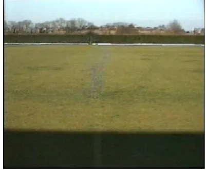
Temporal averaging produces poor results when movement occurs for long periods of time, or if an object lingers in a position for a long period of time. As
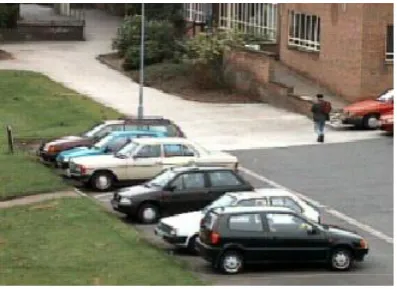
a consequence of the averaging, a „motion blurring‟ effect occurs” [9]. See temporal averaging effect in Fi-gure 2 in comparison with the input image in FiFi-gure 1.
2.3. Temporal Median Filter
“We can extend the principal of the snapshot method to look instead at individual pixels that are steady in value for a specified time, rather than waiting for the entire image to stabilize. The background frame is then created only from pixels that have been stable for more than the specified time. Note that our specification of „stable‟ must allow for some small variation in value to accommodate effects due to noise” [9].
3.
The New Background Algorithm
In this section a new algorithm for background generation is proposed. Firstly, a new method based on temporal median filter is explained in section 3.1. Then a pseudo code is presented in section 3.2. In section 3.3, it will be shown how some parts of the pseudo code should be modified in order to make the method noise tolerant.
3.1. The Method Description
“The algorithm utilizes two bitmaps, BL and BS. BL
holds the background bitmap that will develop as the algorithm processes the incoming frames, and BS holds
the last frame from the camera.
Each pixel in BL has two timers associated with it, TL
and TS. TL is called the long term timer, and counts the
number of frames that a pixel in BL has been steady in
value. Thus as each new pixel value arrives, it is compared to the existing one in BL. If it is within a
tolerance of BL then TL is incremented and the pixel in
BL is replaced with the value of the new pixel.
TS, the short term timer, counts the number of frames
for which the pixel differed from the value in BL. Thus if
a pixel is suddenly covered by a new object, TS will
increase and TL will remain the same. When TS > TL the
pixel has been at the „new‟ value for longer than the value in BL, and so we may assume that the new value is
part of the background. In this case the pixel is copied to BL and BS, and TS is reset to zero.
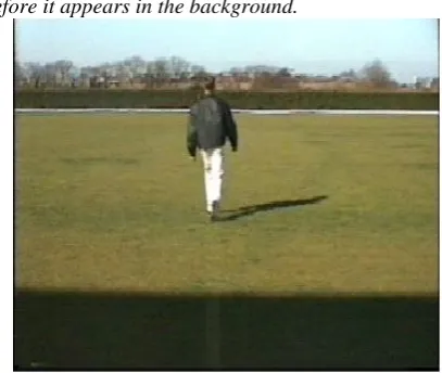
A few additional constraints are required since a limit should be imposed on TL, as the latter could
before it appears in the background.
Figure 1. Image taken by camera (Fld350.bmp).
One further restriction is that TS must be reset to zero
whenever a pixel in the incoming frame is not within of BS . Hence continually changing pixels will not be
incorporated into the background.
The algorithm slowly adapts to changes in the background image (for example the onset of dawn or dusk) as such changes will be within of BL, so BL will
exactly track the slowly changing scene regardless of the value of ” (this method description is from a presentation by Alistair E. May [9]).
3.2. The Pseudo Code of the Algorithm
The algorithm description in section 3.1 can also be presented in pseudo code format as follows:
// The lines preceded by numbers, need some // modifications as will be explained in section 3.3
if (input pixel value [BL − , BL + ] ) {
inc (TL);
1: BL input pixel value;
} else
if (input pixel value [BS−, BS + ] ){
TS 0;
BS input pixel value;
} else{
2: BS input pixel value;
inc (TS );
}
if (TS > TL) {
3: BL input pixel value;
4: BS input pixel value;
Figure 2. Temporal Mean (Mean420.bmp).
TS 0;
}
if (TL > )
TL;
3.3. Temporal Median Filter with Exponentially Weighted Moving Average Filtering
“One advantage of the temporal averaging technique is that noise (which manifests itself as high frequencies) is greatly reduced by the low-pass filter inherent in the method. Reducing the noise in the background image will improve results when we come to perform segmentation.
The temporal median filter cannot reduce noise in this way, but it is easy to rectify it so it does.
At the points in the code of section 3.2 where there is a new incoming pixel, instead of copying it to BS or BL,
we should only add a proportion (e.g., 10%) of the new pixel to a proportion (e.g., 90%) of the existing one. The only exception to this rule is when TS = 0 (and thus
there is a pixel value in BS, which is not the one we wish
to re-use, as it has just changed significantly)” [9]. This effect is called a „simple exponential smoothing filter‟ as it is introduced in [14, chapter 4] and has an updating equation of the form:
BL (x, y, t) (1 − ) BL (x, y, t − 1) + I(x, y, t)
where BL (x, y, t), BL (x, y, t−1) are present and previous
before which the input images are ignored and have no effect on updating of the background image. In fact, it shows how many recent frames should be considered in the updating of the reference image.
Following the above statements, in the pseudo code of section 3.2, the lines preceded by numbers 1 and 3 are replaced by “BL (1 − ) . BL + . input pixel
value” and the lines numbered 2 and 4 are replaced by “BS (1 − ) . BS + . input pixel value” to reduce
the effect of noise.
4. Automatic Parameters Selection
The selection of parameters has a great effect on the performance of the algorithm. In section 4.1 to 4.3 it will be shown how three parameters of the method the exponential smoothing constant , the threshold and the upper limit on TL, i.e., ) should be selected.
4.1. The Selection of
The exponentially weighted moving average (EWMA) is a filter that is used for reduction of the amount of noise in dynamic systems. This filter gives more importance to more recent data by ignoring older data in an exponential manner. The operating characteristics of an EWMA filter are determined by the value of the smoothing constant (0 ≤ ≤ 1). If the value of is large, the smoothing filter output quickly tracks the changes and the fluctuations of input signals. However, if is small, the filter slowly responds to the signal changes. Thus the correct choice of smoothing constant
has an important role on the efficiency of an EWMA filter.
We are interested in choosing the value of depending on the changes of input pixels. “Several techniques have been developed to monitor and modify automatically the value of the smoothing constant in exponential smoothing. These techniques are usually called adaptive-control smoothing methods, because the smoothing parameter modifies or adapts itself to changes in the underlying time series. Trigg and Leach [15] have described a procedure for adaptive control of a single exponential smoothing constant, such as, for example, simple smoothing ST = xT + (1 − ) ST−1 for a constant
process. Trigg and Leach automatically adjust the value of the smoothing constant by setting:
(T) = | Q(T) / ˆ(T) |
Their method is based on the smoothed error tracking signal Q(T)/ˆ(T) where Q(T) is the smoothed
forecast error and ˆ(T) is the smoothed mean absolute deviation, both computed at the end of period T” [14, chapter 9]. The details of the computation of (T) for each pixel are lengthy and are given in the Appendix.
4.2. The Selection of Threshold
“The choice of should be slightly higher than the perturbations in pixel value due to noise. The algorithm is fairly noise tolerant, as a noise impulse on a pixel will temporarily increase TS but not too much so it will rise
above TL. At worst a noise impulse could stop a piece of
the scene from being incorporated into the background. Consider the situation where TS is close to TL, so that BS
contains a pixel that is a good candidate for the background. If a new pixel arrives for this position that deviates by more than from BS due to noise, then TS is
reset and we must wait for frames before the pixel ever has a chance of being incorporated into the background again.
If the value chosen for is too low, then noise will cause problems due to the aforementioned effect. If is too high, then we start to see parts of moving objects appearing in the background, as the algorithm is too insensitive to movement” [9]. Figures 3 to 6 illustrate these effects.
Since the selection of has a great effect on the behavior of the algorithm, a technique is presented here which we will call „noise estimation‟. Thus based on the contents of the images the system can automatically determine a suitable value for and for each color channel separately.
As stated above, should be slightly higher than the noise level. If it is assumed that the noise in the image is of type additive zero mean Gaussian noise, then the standard deviation of noise is an estimate of the noise level for each frame and it is an appropriate choice for the threshold .
A fast estimation of the noise variance for each image can easily be obtained as presented in the paper by John Immerkær [12]. Noise is estimated by using a mask operator N of the form in Figure 7. The mask operator N has zero mean and variance 36n2 assuming
that the noise at each pixel has a standard deviation of
n. If the mask N is applied to
1 -2 1
N = -2 4 -2
Figure 7. Noiseestimation mask operator.
Figure 3. Temporal Median (Tm350.bmp), =1.
Figure 5. Temporal Median (Tm350.bmp), =10.
all pixels of the input image, then the variance of the noise can be computed as:
2 2
image I 1
( ( , ) * N) 36 ( 2)( 2)
n I x y
W H
where I(x, y) denotes the position (x, y) of the input image, and W and H stand for the image width and height, respectively. The standard deviation of the noise should be computed for each color channel separately. The threshold levels are integer values, thus the results obtained are rounded up.
4.3. Choice of
For the choice of , if the video surveillance system is going to operate in indoor or outdoor scenes
Figure 4. Temporal Median (Tm350.bmp), =5.
Figure 6. Temporal Median (Tm350.bmp), =30.
permanently, then any value in the range of a few minutes will work well. Thus the value of 7500 frames (for 5 min) is a reasonable and suitable default value for . However, if the algorithm is being tested offline on a sequence of images consisting of several hundred frames (e.g. 400 to 600 frames), then should be set at least to 10 to 15 percent of the number of frames (i.e., 40 to 60 frames as the minimum value for ).
5. Speed-Up Techniques for Computing
the Parameters
5.1. A Speed-Up Technique for the Computation of
computations of smoothed constant (T) for each pixel, we use the following technique:
If the absolute difference between the input pixel intensities and the previous pixel intensities is less then or equal to 2, use the previous values of (T) for the new input pixel (i.e., all those computations for Q(T) and ˆ(T) that lead to the computation of (T) for each color channel are not needed to be accomplished).
Since many pixels have almost the same intensities in two or three successive frames, a significant reduction in the number of calculations for (T) could be achieved.
For implementing this technique, we just need to keep a previous image in memory. For each input pixel, we compare the pixel intensities in three color-channels with its corresponding pixel intensities in the previous image. If for either color channel, the absolute difference between input pixel intensity and the previous pixel intensity is greater than 2, the computation of (T) is done for all three channels and the input pixel intensities are copied to the previous image. Thus, after processing several frames, previous image pixel intensities would be obtained from different frames.
The quality of background images using this speed-up technique is very similar to the quality of reference images obtained based on the full computation of (T) for all the pixels. However, the experiments show this technique reduces on the average about 20 percent the processing time of computation of (T) for each frame (e.g. 60 ms is reduced to 50 ms).
5.2. A Speed-Up Technique for the Computations of the Thresholds
We use „noise estimation‟ method to compute the noise level for three color channels and each frame separately. However, the noise level is often due to camera noise that is fixed for all frames. Thus one of the following techniques can be used for speeding up the computation of threshold for each color channel:
„Noise estimation‟ can be applied to a number of initial images to compare the threshold levels for three color channels of successive frames. If the threshold levels of corresponding color channels are the same, we can use those threshold levels for all the input images. In this case, no time is spent for the computation of threshold for the remaining input images.
If the threshold levels change but very rarely (e.g. due to rounding up) or if we want to be more conservative by assuming that the camera noise level
may change suddenly, for example, by fluctuating the environment lighting condition, we can still apply „noise estimation‟ method first to red channel for frame „i‟, then to green channel for frame „i + 1’ and finally to blue channel for frame „i + 2’. This process can be repeated for all the succeeding frames and previous values of threshold levels are utilized for the other two channels. This speed-up technique can reduce the computation time for at least 5 to 10% in comparison with the computation of threshold levels for all three channels.
6. Experimental Results and Analysis
Using an adaptive-control smoothing method for the computation of is justified in section 6.1. In section 6.2 the results of applying the algorithm to several sequences of images are shown and the results are analyzed.
6.1. Justification for Using an Adaptive-Control Smoothing Method for the Computation of
In section 4.1 and in the Appendix, the Trigg and Leach‟s adaptive-control smoothing method [15] was explained. In addition, in section 5.1, a speed-up technique for the computation of (T) was offered. A possible question that may be asked is the reason for using such lengthy computations for rather than using a fixed (e.g. = 0.1). There are two main reasons that justify the application of adaptive-control method as pointed out below:
1. The adaptive-control smoothing method has the capability of removing the effect of simulated noise faster than the best fixed- value provided that after a specified number of frames including simulated Gaussian noise, there are a number of succeeding frames containing no simulated noise.
2. The foreground objects‟ residues are removed more quickly and the background image is obtained more rapidly using adaptive-control smoothing method in comparison with the best fixed- value for the same number of frames.
In order to show point 1, the following experiments were accomplished:
Figure 8. Back_Img212.bmp, Differ1 = 7993114.
of fixed minimizes | Back_Img180 – Fld180 | where Back_Img180 is the generated background image for Fld′180 and Fld180 is the real background image. The value of = 0.96 was obtained for all the simulated noisy frames regardless of the standard deviation of the simulated noise.
It means that if a fixed value of (e.g. the optimal value) is used, the same result is yielded independent of the standard deviation of the simulated noise. Of course, it is easy to show mathematically that in the following formula
BL (x, y, t) (1 − ) BL (x, y, t − 1)+ I (x, y, t)
if we assume that the camera noise plus simulated Gaussian noise in BL (x, y, t − 1) and I (x, y, t) are
almost the same, then regardless of the value of , the same total amount of noise is produced in BL (x, y, t).
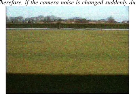
After Fld′80 to Fld′180 containing simulated Gaussian noise with standard deviation of = 4.0, we added Fld181 to Fld212, a number of input frames from the background scene including no moving objects. The previous experiment was performed but on the total sequence Fld′80 to Fld212 for the optimal value of fixed that minimizes difference1 | Back_Img212 − Fld212 | where Back_Img212 (Fig. 8) is the generated background image after operating on the total sequence and Fld212 is the real background image. The value of = 0.25 was obtained as the result. Then the algorithm was run with the adaptive-control smoothing method on the same total sequence and difference2 | Adaptive_Back_Img212 – Fld212 | was also computed where Adaptive_Back_Img212 is the generated background image using adaptive-control smoothing method (see Fig. 9). The experiment showed that difference2 is smaller than difference1.
Therefore, if the camera noise is changed suddenly due
Figure 9. Adaptive_Back_Img212.bmp, Differ2 = 7201674.
to any unknown reason almost rarely and after some number of frames the camera noise gets back to its normal level, the adaptive-control smoothing method is more capable to remove the effect of the extra noise with a fewer number of frames than with the fixed value. The reason is that, although this is an important feature of the exponentially weighted moving average (EWMA) filter to place more emphasis on most recent data, however, selection of larger smoothing constant automatically gives even more importance to the current input data than with the fixed and thus better results are yielded.
If the camera noise is never changed, there is still an even more important feature of the adaptive-control smoothing method as mentioned in the case 2 above. To demonstrate this feature, the following experiment was done:
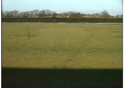
Consider a sequence of input images Fld250 to Fld350 containing a moving object. We repeated the algorithm on this sequence to find the optimal fixed that minimizes difference1 | Back_Img350 – Fld212 | where Back_Img350 (Fig. 10) is the generated background image for Fld350 and Fld212 is the closest and most recent real background image available for image Fld350, since Fld350 includes a moving object. The result = 0.50 was obtained. Then adaptive-control smoothing method was also run on the same sequence and difference2 | Adaptive_Back_Img350 – Fld212 | was also computed where Adaptive_Back_Img350 is the generated background image using adaptive-control smoothing method for Fld350 (Fig. 11). The experiment showed that difference2 is smaller than difference1.
on the quality of background images. In fact, if an
Figure 10. Back_Img350.bmp, Differ1 = 3102308.
Figure 12. Field Noise Estimation (Fld_Ne248.bmp) Red- = 3, Green- = 3, Blue- = 3 (size: 384 × 288) Computation Time = 57 ms.
Figure 14. Field Noise Estimation (Fld_Ne315.bmp) Red- = 3, Green- = 3, Blue- = 3 (size: 384 × 288) Computation Time = 58 ms.
adaptive-control smoothing method is not used, the reference images will not be obtained in such a few numbers of frames with most of the foreground pixels
removed.
Figure 11. Adaptive_Back_Img350.bmp, Differ2 = 2732747.
Figure 13. Field Noise Estimation (Fld_Ne275.bmp) Red- = 3, Green- = 3, Blue- = 3, (size: 384 × 288) Computation Time = 56 ms.
6.2. Analysis of Results
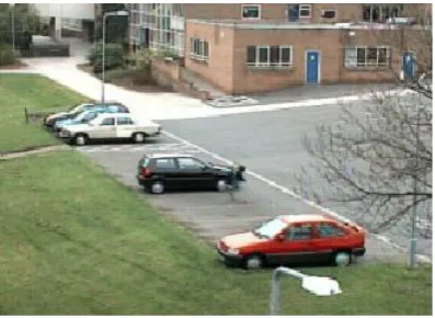
Figures 12 to 15 show how rapidly the foreground object pixels are removed from the reference frames while there is a moving object. In fact, the algorithm usually needs 6 to 10 s (less than 250 frames, based on 25 frames/s) to find the background frame where there are moving objects included and it needs less than 2 s (50 frames) if the algorithm starts with 40 to 50 images that demonstrate the environment‟s lighting condition is changing (i.e., not static images) but there isn‟t any moving object in them. Thus, these numbers of frames are enough for the algorithm to find the background images from that frame on although there are a number of moving objects appearing in the succeeding input images.
At the present time, 17 to 18 color images (with the resolution of 384 × 288 pixels and processing time of 55 to 56 ms. on the average for each image) are processed on a 1.7 GHz Pentium 4 PC with 1GB of RAM running Windows 2000 Professional Edition (the images shown above are almost half of the size of the original images in order to take less space). If standard images (i.e., 320 × 240 pixels) are used, processing time can at least be reduced by the value of 1.44 (384 × 288 / 320 × 240), yielding processing rate of 25.7 to 26.2 Hz (38.2 to 38.9 ms. for each frame). This shows that the algorithm can run in real time on a Pentium 4 PC for standard images (due to 25 input frames/s, the processing time for every frame should be less than 40 ms). Meanwhile, upon appearing faster PCs (with higher CPU speeds) at the market, more processing rate is readily feasible. Thus, in the near future, the algorithm can run in real time even for images with relatively high resolutions (such as 384 × 288 pixels).
We have examined the proposed algorithm on different sequences of images and almost in all the cases it has performed quite fast and well with
encouraging results confirming the robustness of the algorithm for color images (see Figs. 16 to 23).
7. Conclusions and Future Work
A new real-time dynamic background generation technique for color images taken from a static camera was presented. Initially, three existing methods called snapshot, temporal averaging and temporal median filtering were evaluated. Then based on the strengths and the weaknesses of these methods, the final algorithm called „temporal median filter with exponentially weighted moving average (EWMA)‟ was introduced.
One of the advantages of the new algorithm is that two of its parameters are computed automatically. In contrast to some other background generation techniques, the new algorithm does not need to have any training period for initializing the parameters [5]. In fact, after the first input frame that is used for the long-term bitmap (i.e., BL), the dynamic background image is
generated for the second and all the succeeding frames. In addition, the method could start its operation for a sequence of images in which moving objects are included. Finally, from the results obtained, the algorithm was shown to be fast, robust and efficient (from the Figs. 12 to 23, it is obvious that all moving pixels have been removed thus the algorithm is robust and it takes less than 125 frames (for Figs. 20 to 23 about 50 frames) for background generation).
We have found that about 70% of the computation time of the new algorithm is spent calculating (the constant of EWMA). It is possible to find some shortcuts such as lookup tables so that the value of is found using a table rather than performing lengthy computations (of course, interpolations might be used for the values not listed in the lookup table).
Figure 17. Car_Park3 Input Image (Cp3_115.bmp) (size: 352 × 288).
Figure 18. Car_Park3 Noise Est. (Cp3_Ne70.bmp) Red- = 5, Green- = 5, Blue- = 6, (size: 352 × 288) Computation Time = 51 ms.
Figure 20. Car_Park1 Input Image (Cp1_333.bmp) (size: 352 × 288).
Figure 22. Car_Park1 Noise Est. (Cp3_Ne345.bmp) Red- = 6, Green- = 5, Blue- = 6 (size: 352 × 288) Computation Time = 53 ms.
Figure 19. Car_Park3 Noise Est. (Cp3_Ne115.bmp) Red- = 5, Green- = 5, Blue- = 6 (size: 352 × 288) Computation Time = 52 ms.
Figure 23. Car_Park1 Noise Est. (Cp3_Ne383.bmp) Red- = 6, Green- = 5, Blue- = 6 (size: 352 × 288) Computation Time = 52 ms.
As for future work, more research should be done so that a separate threshold level is computed for each pixel with very short computation time and efficient result. An individual threshold for each pixel is more robust than using a single threshold for all the pixels in each color channel.
Finally, if the system needs to operate continuously, the value of might be chosen dynamically based on the contents of images. However, more investigations should be done to determine whether changing the value of might have a positive effect in the efficiency of the algorithm when it is used for long periods of time.
Acknowledgments
Mr. Bijan Shoushtarian wishes to acknowledge the financial support of the University of Isfahan and the Ministry of Science, Research and Technology (MSRT) of Iran for his doctoral scholarship.
References
1. Wren C., Azarbayejani A., Darrell T., Pentland A. Pfinder: Real-time tracking of the human body. IEEE Trans. Pattern Analysis and Machine Intelligence, 19(7): 780-785 (1997).
2. Haritaoglu I., Harwood D., and Davis L.S. W4: Who? When? Where? What? A Real Time System for Detecting and Tracking People. Proc. of the Third International Conference on Automatic Face and Gesture Recognition (FG‟ 98), April (1998).
3. Horprasert T., Haritaoglu I., Wren C., Harwood D., Davis L.S., and Pentland A. Real-time 3D Motion Capture. Proc. of 1998 Workshop on Perceptual User Interfaces (PUI‟ 98), Nov. (1998).
4. Elgammal A., Harwood D., and Davis L.S. Non-parametric Model for Background Subtraction. ICCV Frame Rate Workshop, Sept. (1999).
5. Horprasert T., Harwood D., and Davis L.S. A Statistical Approach for Real-time Robust Background Subtraction and Shadow Detection. ICCV Frame Rate Workshop, Sept. (1999).
6. KaewTraKulPong P. and Bowden R. An Improved Adaptive Background Mixture Model for Realtime Tracking with Shadow Detection. In Proc. 2nd European Workshop on Advanced Video Based Surveillance Systems, AVBS01. VIDEO BASED SURVEILLANCE SYSTEMS: Computer Vision and Distributed Processing, Kluwer Academic Publishers, Sept. (2001).
7. Grimson W.E.L., Stauffer C., and Romano R. Using adaptive tracking to classify and monitor activities in a site. In Proceedings. 1998 IEEE Computer Society Conference on Computer Vision and Pattern Recognition (Cat. No.98CB36231). IEEE Computer Soc. (1998). 8. Grimson W.E.L. and Stauffer C. Adaptive background
mixture models for real-time tracking. In Proceedings. 1999 IEEE Computer Society Conference on Computer Vision and Pattern Recognition (Cat. No PR00149). IEEE Computer. Soc., Vol. 2 (1999).
9. May A.E. Background Generation. Internal Department Presentation. Dept. of Computer Science, Loughborough University (1998).
10. Rosin P.L. and Ellis T. Image difference threshold strategies and shadow detection. In British Machine Vision Conf., pp. 347-356 (1995).
11. Dawson-Howe K.M. Active surveillance using dynamic background subtraction. Trinity College, Dublin, Ireland, Aug. (1996).
12. Immerkær J. Fast noise Variance Estimation. Computer Vision and Image Understanding, 64(2): 300-302 (1996). 13. Rosin P.L. Thresholding for Change Detection.
Proceedings of International Conference on Computer Vision (1998).
14. Montgomery D.C., Johnson L.A., and Gardiner J.S. Forecasting & Time Series Analysis. 2nd Edition, McGraw-Hill, Inc. (1990).
15. Trigg D.W. and Leach A.G. Exponential smoothing with an adaptive response rate. Operational Research Quarterly, 18(1): 53-59 (1967).
Appendix
As stated in section 4.1, “Trigg and Leach [15] automatically adjust the value of the smoothing constant by setting:
(T) = | Q(T) / ˆ(T) | (9.4)1 their method is based on the smoothed error tracking signal
Q(T) / ˆ (T) (9.1)
where Q(T) is the smoothed forecast error and ˆ(T) is
1
the smoothed mean absolute deviation, both computed at the end of period T. The smoothed error is computed according to
Q(T) = e1(T) + (1 – ) Q(T – 1) (9.2)
where Q(0) 0 and the smoothed mean absolute deviation is
ˆ
(T) = | e1(T) | + (1 – ) ˆ(T – 1) (9.3)
where e1(T) is the forecast error in period T and is
smoothing constant such that 0 < < 1.” [14, chapter 9].
“In contrast to Q(0) that is zero, ˆ(0) 0. However, ˆ
(T) can be obtained based on an estimate of the standard deviation of the single-period-ahead forecast error, i.e., e(T), where e2 Var [e1(T)]2 as follows:
ˆ
(T) = e(T) / 1.25 (8.9) An estimate of the variance of the single-period-ahead forecast error can be computed using the sample variance of the last N forecast errors:
21 1
2 = +1
e (t) e (T) σ (T)=
1
N
Tt T N
e (8.7)
where e1(T) is the average of the last N errors and is
defined as follows” [14, chapter 8, with some sentences modified]:
1 1
= +1
1
e (T) e (t)
N
T
t T N
(8.5)
“The 1-period-ahead forecast error for the period T is defined as:
e1 (T) = xT – ˆX(T – 1) (7.6)
where xT is the input value and ˆX(T – 1) is the forecast
value for period T computed at the end of period T – 1” [14, chapter 7, with a sentence modified].
“Suppose we know that the average level of the input values do not change over time or it changes very slowly. In this case, a simple exponential smoothing for
a constant process can be developed and it might be modeled as:
x t = b + t
where b is the expected input value in any period and t
is a random component having mean 0 and variance
2. Thus it can be shown that the forecast for input
value in any future period T + would be
xT+ = ST (4.6)
where ST is an estimator for the unknown parameter b
in the constant process. ST is shown to obtain using the
following equation:
ST = xT + (1 – ) ST – 1 (4.1)
by assuming S0 = x0. Equation (4.1) is called „simple
exponential smoothing‟ and ST is called smoothed
statistic. The fraction is also called the smoothing constant.” [14, chapter 4, with some sentences modified].