Stabilization of Networked Control Systems with Variable
Delays and Saturating Inputs
M. Mahmodi Kaleybar* and R. Mahboobi Esfanjani* (C.A.)
Abstract:In this paper, less conservative conditions for the synthesis of static state-feedback controller are introduced to stabilize networked control systems subject to actuator saturation. Both of the data loss and latency which deteriorate the performance of the closed-loop system are modeled as the variable delays. Two different techniques are employed to import actuator saturation in the controller design procedure. The novelty of the proposed schemes is to utilize an improved Lyapunov-Krasovskii functional, free-weight matrix and parameter tuning method to obtain more efficient conditions to determine state-feedback gain for a constrained system which is controlled over the communication network. Moreover, optimization problem is formulated in order to find the largest possible estimate for the region of attraction corresponding to maximum allowable delays. Numerical examples are presented to demonstrate the outperformance of the suggested approaches compared to the existing results in the literature.
Keywords: Input Saturation, Linear Matrix Inequality (LMI), Networked Control Systems, Variable Delay.
1 Introduction1
Networked Control System (NCS) is a feedback structure wherein the control loop is closed through a communication network. The advantages of NCSs such as low cost and simple installation and maintenance make them more and more popular in many real-world applications including industrial automation and multi-agent systems [1]. However, the presence of communication network in the control loop complicates the analysis and design of the control system. Main issues are the delay and dropout of data packets which occur when sensors, actuators and controller exchange information across the network. The design of NCSs with considering the effects of data delay and dropout has been studied by many researchers [2-4]. On the other hand, physical constraints, especially actuator saturation are encountered in practical systems [5]. So, the input saturation in the analysis and synthesis of time-delay systems has attracted recently many attentions [6-16].
In [6], stabilizing controller was designed for NCSs with actuator saturation and sampling period variation. A continuous functional whose values at the sampling instants coincides with a discrete-time Lyapunov
Iranian Journal of Electrical & Electronic Engineering, 2014. Paper first received 7 Aug. 2013and in revised form 18 Feb. 2014. * The Authors are with the Department of Electrical Engineering, Sahand University of Technology, Tabriz, Iran.
E-mails: [email protected] and [email protected].
function is utilized to derive sufficient condition in terms of linear matrix inequality (LMI) for computing the stabilizing controller. In [7], stabilization problem of networked stochastic systems subject to actuator saturation was studied. The nonlinearity of actuator saturation was modeled as a convex polytope of linear systems. In [8], the problem of designing state-feedback stabilizing controller and enlarging the controller domain of attraction is formulated as an optimization problem with LMI constraints. In [9], simple sufficient LMI conditions are derived for stabilization of systems with polytopic uncertainty for regional stabilization of systems with sampled-data saturated state-feedback via descriptor approach. The regional stabilization and H∞
control problem have been studied in [10] by combining the descriptor model transformation and Moon's inequality which is used to get a less conservative bound for the cross terms. Using a new Lyapunov-Krasovskii functional and generalized sector relation, conditions were extracted in [12] for the controller design, aiming at the enlargement of the region of attraction, as well maximizing the upper bound of the sampling period. In [13], stabilization problem of neutral delay systems in the presence of control saturation is solved based on the descriptor approach and the use of a modified sector condition.
This paper presents less conservative procedures to synthesis asymptotically stabilizing state-feedback controller for networked control systems subject to
actuator saturation. The NCS model developed in [2] is adopted and the nonlinearity of actuator saturation is tackled in two ways: In the first approach, the saturation is represented by a convex polytope of linear systems. In the second scheme, generalized sector condition (decentralized dead zone nonlinearity) is used to handle the saturation effects. The key ideas in the proposed methods are first, to use an improved Lyapunov-Krasovskii functional and second, to utilize the free-weight matrix and parameter tuning methods for extracting improved conditions to obtain the controller gain for networked systems with saturating input, aiming at enlarging the estimate of the region of attraction and maximizing maximum allowable delay bound.
A challenging issue in the controller synthesis for the nonlinear processes is stabilizing the closed-loop systems while achieving the largest possible domain of attraction, i.e. enlargement the set of initial states for which the asymptotic convergence of the system trajectories to the origin is ensured. Thus, in this note, a computationally tractable optimization problem with LMI constraints is formulated to find a less conservative estimate for the domain of attraction. Simulation results demonstrate that the designed controller leads to larger domain of attraction while increases the maximum allowable delay bound.
The paper is organized as follows: In section 2, the NCS model is described and then the problem of interest is explained. Section 3 presents some preliminary facts which will be used in the derivation of the main results of the paper. The proposed procedures to determine controller gain, maximum allowable delay and domain of attraction are derived in section 4. In section 5, numerical examples are given to illustrate the superiority of the proposed methods compared to the existing results in the literature. Section 6 concludes the paper.
Notations: ℜn denotes the ndimensional Euclidean
space with vector norm and ℜn m× is the set of all n×m real matrices. The notation P>0 (P≥0) means that P is symmetric and positive definite (positive semi definite). The subscript T
stands for matrix transposition. Co{} symbolizes the convex hull. diag{} is used as an ellipse for block-diagonal matrix. ( )σ denotes the largest singular value of the matrix. The symbol * shows the symmetric entry in a symmetric matrix. Finally, the space of continuously differentiable vector function over [-η, 0] is represented by C1[-η, 0].
2 Problem Statement
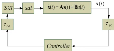
A typical networked control system is shown in Fig. 1, wherein the controller, sensor and the actuator are assumed to be separated and connected through a communication network. The controlled system is linear and time invariant, sensor is time-driven and controller and actuator are event-driven. In the considered
network, all the data are lumped together into one packet and transmitted at the same time (single packet transmission) and the sent packets are time stamped. The controller and actuator always use the new data packets and discard the old ones. When an old data packet arrives, it is dealt with as a packet loss. A zero-order-hold is placed in the input of the plant and the input is zero before the first controller packet arrives.
Regarding the above assumption on the NCS, the following equations can describe the closed-loop system behavior:
( )t = ( )t + ( )t
x A x Bu (1)
1
1
( ) sat(t = (t−τik) ), t∈[i hk +τik,i hk+ +τik+ )
u K x (2)
where x( )t ∈ ℜn and u( )t ∈ ℜm are the state and the
control vectors, respectively. A and B are two constant matrices with appropriate dimensions. K is the state feedback gain matrix. h stands for the sampling period. k = 1, 2, 3,…is the number of the controls which act on the system, ik is an integer denoting the sampling instant of the state feedback corresponding to the k-th effective control. Transmission delay and loss induced by the network is composed of two parts: sensor-to-controller
sc
τ and controller-to-actuator τca. Since the controller
is static, these two values can be lumped together as ,
k
i sc ca
τ =τ +τ where time-varying τik represents the
network-induced delay and dropout at the instant ikh. The function sat( ):⋅ ℜ → ℜm m denotes standard
saturation: sat ( ) sign ( ) min ( ,ui = ui u ui i ) with
max( ).
i i
u = u
The closed-loop system model in Eqs. (1)-(2) can be represented as x( )t =A x( )t +Bsat(K x(i hk ) ) for
1
1
[ , )
k k
k i k i
t∈ i h+τ i h+ +τ + . Now, by definition of
( )t t i hk
τ = − ,t∈[i hk +τik,i hk+1 +τik+1), this relation can
be rewritten as Eq. (3):
( )t = ( )t + sat( (t−τ( )) )t
x A x B K x (3) which is a continuous-time system with delayed input. Note that the varying delay is bounded as follows:
1
1
0≤τik ≤τ( )t ≤(ik+ −i hk) +τik+ ≤η (4)
ZOH
x
(
t
)
=
Ax
(
t
)
+
B
u
(
t
)
x(t)Controller
sc
τ
ca
τ
sat
sat
Fig. 1 Schematic Diagram of the Saturated NCS.
Furthermore, the initial condition for system of Eq. (3) is a continuous differentiable function which is shown as the following:
( ),
φ θ =
0
x θ∈ −[ η, 0] (5) Briefly, the NCS is modeled as the nonlinear time-delay system in Eq. (3), wherein the variable time-delay characterized in Eq. (4) represents both of the data loss and latency in the network. The problem of interest is to determine the state-feedback gainK such that the controller in Eq. (2) renders the closed-loop system of Eqs. (1)-(2) asymptotically stable; as well an estimate of the domain of attraction is obtained.
3 Preliminaries
In this section, some useful facts which are needed to solve the explained problem are recalled. First, the stability theorem of time-delay system is presented and afterward, essential definitions and relations to formulate the actuator saturation are reviewed.
Theorem (Lyapunov-Krasovskii): Suppose that f maps a bounded set fromC1[-η, 0] into a bounded set
into ℜn, and
1, 2, 3: 0 0
α α α ℜ → ℜ≥ ≥ are continuous, non-decreasing functions with α1(0)=α2(0)=α3(0)=0
andα1(s)>0, α2(s)>0 for s>0. If there exists a continuous
functional 1
0
: [ , 0]
V C −η → ℜ≥ such that
1 2 3
[ ,0]
( (0) ) ( sup ( ) ), ( ( ) )
t
x V x t V x t
η
α α α
∈ −
≤ ≤ < − (6)
Then the equilibrium of Eq. (3) is stable. If, in addition, α3(s)>0 for s>0, then it is asymptotically
stable.
Definition 1 [17]: Let ki be the ith row of the
matrix K, a polyhedron region ( )L K in the state space is defined as follows:
{
}
( ) n: , 1, 2, ,
i i
L K = x∈ℜ k x ≤u i= " m . (7) Furthermore, an ellipsoid E in the state space is characterized as the following:
( ,1) { n: T 1}
E P = ∈ℜx x Px≤ (8) wherein, P∈ ℜn n× is a positive definite matrix.
Definition 2 [17]: The set
ν
consists of all m m×diagonal matrices whose diagonal elements are either 1 or 0; so, the number of members in
ν
are 2m. Let thematrix , 1, 2, , 2m j
D j= " be a member of the set
ν
, and define: Dj I Dj− = − . It is clear that the matrix
j
D− is also a member of
ν
, i.e. D Dj, j−∈ν .In the Lemma 1, based on the definitions 1 and 2, the saturation function of vectors belong to a polyhedron region is described as a convex combination of well-defined vertices.
Lemma 1 [17]: Let K H, ∈ ℜm n× are given; for all ndimensional vector x∈L( )H , the following holds:
sat ( ) { , 1, , 2 }m
j j
Co D D− j
∈ + =
K x K x H x " (9)
Hence, sat (K x)can be expressed as follows:
2
1
sat( ) ( )
m
j j j
j
D D
λ −
=
=
∑
+K x K H x (10)
in which,2
1
1 m
j j
λ
=
=
∑
and λj ≥0.Definition 3 [18]: Decentralized dead-zone nonlinearity is the vector function ψ which is defined as follows:
( ) sat( )
ψ Kx =Kx− Kx (11)
Lemma 2 [18]: Consider the function
( )
ψ Kx defined in Eq.(11). For x∈ ℜn if x∈L(K H− ),
the following is hold:
( ) ( ( ) ) 0
T
ψ Kx Uψ Kx −Hx ≤ (12) for any diagonal positive definite matrix U∈ ℜm m× .
The result of Lemma 2 which is known as generalized sector condition will be utilized later to transform the design conditions into LMI form.
Definition 4: Let ϕ( , )t x0 be the state trajectory
ofthe system of Eq. (3), starting from the initial function
1[ , 0]
C η
∈ −
0
x ; the domain of attraction of the origin is defined as the following:
1
{ [ , 0] : lim ( , ) 0 }
t
S C η ϕ t →∞
= x0∈ − x0 = (13) Furthermore, an estimate of the domain of attraction
DOA S
Χ ⊂ can be obtained as follows:
{
:max | | 1, max | | 2}
DOA S δ δ
Χ = x0∈ x0 ≤ x0 ≤ (14) by maximizing positive scalars δi(i=1, 2).
4 Main Results
In this subsection, the sufficient conditions are derived to determine state-feedback gain to asymptotically stabilize the system of Eq. (3). Based on the convex representation of saturation function in Lemma 1, design condition is introduced in Theorem 1 to obtain the controller gain. The result of Theorem 1 is used in Corollary 1 to determine the largest possible estimate of the domain of attraction. In Theorem 2, using the property of decentralized dead zone nonlinearity in Lemma 2, another criterion is derived to obtain the controller gain and corresponding domain of attraction.
Theorem 1: Given scalars η>0 and p ii, =2, 3, 4
the system of Eq. (1) with the networked memoryless state-feedback controller in Eq. (2) is asymptotically
stable if there exist matrices P P = T >0, Q Q = T >0,
0,
T
= >
R R G Y, and nonsingular matrix
1 2 2
T
= + +
Φ Ω Ω Ω of appropriate dimensions such that the following matrix inequalities hold:
0, j 1, 2,..., 2m
< =
Φ (15)
0, 1, 2,..., * s s s u s m u ⎡ ⎤≥ = ⎢ ⎥ ⎣ ⎦ g
P (16) where Φ Ω = 1+Ω2+ΩT2 with:
1 2 * 2 * * * * * η ⎡ − ⎤ ⎢ ⎥ − ⎢ ⎥ =⎢ ⎥ ⎢ ⎥ − − ⎢ ⎥ ⎣ ⎦
Q R R P 0
R 0 R
Ω R 0 Q R (17)
2 2 2
2
3 3 3
4 4 4
( ) ( ) ( ) ( ) T T j j T T j j T T j j T T j j D D
p p D D p p p D D p p p D D p
− − − − ⎡ − − + ⎤ ⎢− − + ⎥ ⎢ ⎥ = ⎢− − + ⎥ ⎢ ⎥ − − + ⎢ ⎥ ⎣ ⎦
A X B Y G X 0
A X B Y G X 0
Ω
A X B Y G X 0
A X B Y G X 0
(18)
and gs is the s-th row of G; Furthermore, K Y X= −T
and H G X= −T. An estimate of the domain of attraction is in the form of Eq. (14) with δ1 and δ2 satisfying:
(
)
2 1 1
1
3
2 1
2
( ) ( )
( ) 1
2
T T
T
δ σ η σ
η δ σ
− − − −
− −
+
+ ≤
X P X X Q X
X R X
(19)
Proof: Regarding the Lemma 1, the closed-loop system in Eq. (3) is represented as a more tractable form of Eq. (20):
2
1
( ) ( ) ( ) ( )
m
j j j k
j
t t λ D D− i h
=
= +
∑
+x A x B K H x (20)
provided that x∈L( )H , wherein 0≤λj ≤1and
2 1 1 m j j λ = =
∑
. Therefore, the system equation in vertex j is as follows:( )t = ( )t + j (i hk )
x Ax A x (21) in which Aj =B(DjK+Dj−H) for j=1, ,2" m.
In what follows, the derivative of an appropriate energy functional on every vertex of the system, represented in Eq. (21) is set to be negative. Improved Lyapunov-Krasovskii functional candidate is considered as follows:
( ) T( ) ( ) t T( ) ( )
t
V t t t η s s ds −
=x P x +
∫
x Q x0
( ) ( )
t T t
s s ds d η θ
η θ
− +
+
∫ ∫
x Rx (22)in which, P P= T >0, Q Q= T >0 and R R= T >0 are
to be determined. Calculating the time derivative of
( )
V t along the trajectories of the system of Eq. (21) yields to:
2
( ) 2 ( ) ( ) ( ) ( ) ( ) ( )
( ) ( ) ( ) ( )
T T T
t
T T
t
V t t t t t t t t t s s ds
η η η η η − = + − − − + −
∫
x Px x Qx x Qx
x R x x R x
(23)
To obtain design condition in terms of matrix inequalities, first, a quadratic upper bound is derived for the integral term in ( )V t . To this end, the following relation is used:
( ) ( ) ( ) ( ) ( ) ( ) k k t T t
i h t
T T
t i h
s s ds
s s ds s s ds η η η η η − − − = − −
∫
∫
∫
x R x
x R x x R x
(24)
On the other hand, regarding the Jensen Lemma [3], the following inequalities hold:
( ) ( ) [ ( ) ( )] [ ( ) ( )] k t T i h T k k
s s ds
t i h t i h
η
− ≤
− − −
∫
x Rxx x R x x
(25) ( ) ( ) [ ( ) ( )] [ ( ) ( )] k i h T t T k k
s s ds
i h t i h t η η η η − − ≤ − − − − −
∫
x Rxx x R x x
(26)
So, substituting Eqs. (25) and (26) in Eq. (24) results in the following upper bound for ( )V t :
2
2 ( ) ( ) ( ) ( ) ( ) ( )
[ ( ) ( )] [ ( ) ( )]
( ) ( ) [ ( ) ( )] [ ( ) ( )]
T T T
T
k k
T T
k k
V t t t t t t
i h t i h t
t t t i h t i h
η η η η η ≤ + − − − − − − − − + − − −
x Px x Qx x Qx
x x R x x
x Rx x x R x x
(27)
Now, let us define
[
]
( ) ( ), ( ), ( ), ( ) T k
t = t i h t t−η
ξ x x x x ; it is obvious that
for any matrix M, the following relation is true:
2 ( ) [ ( )T ( ) ( ) ( )] 0
j j k
t t − t − D +D− i h =
ξ M x Ax B K H x (28)
It should be noted that M is a free-weight matrix which is injected in upper bound of ( )V t to increase the degree of freedom in the final design condition to reduce the conservativeness of the obtained sufficient criterion. Adding Eq. (28) to Eq. (27) and arranging the obtained relation yields to:
( ) T ( ) ( )
V t ≤ξ t Φ ξt (29)
where Φ Ω= 1+Ω2+Ω2T and
1 2 * 2 * * * * * η − ⎡ ⎤ ⎢ − ⎥ ⎢ ⎥ = ⎢ ⎥ ⎢ ⎥ − − ⎣ ⎦
Q R R P 0
R 0 R
Ω
R 0
Q R
(30)
2 = −⎡⎣ − (Dj +Dj− ) ⎤⎦.
Ω MA MB K H M 0 (31)
If Φ <0, the Lyapunov-Krasovskii Theorem ensures that the system of Eq. (21) and consequently, the system of Eq. (20) is asymptotically stable. The inequality condition Φ<0 is a nonlinear matrix inequality which is transformed to LMI by changing variable technique. For this purpose, first, the matrix
Mis partitioned as follows:
1 2 3 4
T
T T T T
⎡ ⎤
= ⎣ ⎦
M M M M M (32)
Afterward, let M1=M0, M2=p2M0, M3=p3M0,
M4=p4M0,X=M01
− and Z=diag(X,X,X,X). Define:
1 2 2
T T
= = + +
Φ ZΦZ Ω Ω Ω , wherein,
T
i = i
Ω ZΩZ for i = 1, 2, P =X P XT, Q =X Q XT,
,
T T
= =
R X R X Y K X and G=H XT. The
inequality Φ <0 implies that Φ<0. Briefly, this proves the sufficiency of the condition of Eq. (15) to asymptotic stability of the closed-loop system.
Employing the Lemma 1 to derive Eq. (20) requires that x∈L( )H is assured. In the following, condition is derived to guarantee the belonging of the state to the mentioned region. Let the ellipsoid ( ,1)E P is a subset of the region ( )LH , so the following inequality is satisfied:
2 ( 1 T ) 2 , 1, ,
i ≤ ui + ≤ ui i= m
h x x P x " (33)
Since:
[
]
12 (1 ) 1 0
*
i i
T
i i
i
u u
u
⎡ ⎤ ⎡ ⎤
≤ + = ± ⎢ ⎥ ⎢ ⎥≥
± ⎣ ⎦
⎣ ⎦
h
h x x P x x
P x (34)
The following holds: 0
* i i
i
u u
⎡ ⎤
≥
⎢ ⎥
⎣ ⎦
h
P (35)
If both sides of the above inequality pre and post multiplied simultaneously with diag( , )I X and its transpose respectively, the inequality of Eq. (16) is
obtained with T
i = i
g h X .
Finally, an estimate of the domain of attraction in the form of Eq. (14) is computed. From ( ) 0V t < , it follows that V( )xt <V( )x0 and therefore for t>0:
0
( )T ( ) ( ) ( )
t
t t < V < V
x P x x x (36) Regarding Eq. (14), the following inequalities hold:
2
0 [ ,0]
3 2 [ ,0]
3
2 2
1 2
( ) max ( ) ( ( ) ( ))
max ( ) ( )
2
( ( ) ( )) ( )
2
V
θ η
θ η
φ θ σ ησ
η
φ θ σ
η
δ σ ησ δ σ
∈ −
∈ −
≤ +
+
≤ + +
x P Q
R
P Q R
(37)
So, if:
3
2 2
1 ( ( ) ( ) ) 2 2 ( ) 1
η
δ σ P +η σ Q + δ σ R ≤ (38)
then, for all the initial functions belong to ΧDOA in Eq.
(14), the trajectories of the closed-loop system remain in the ellipsoid ( ,1)E P ⊂L( )H and the polyhedron representation of saturation function is valid.
Theorem 1 gives a systematic approach to determine controller gain K via feasible solution of inequalities in Eq. (15) and Eq. (16) after tuning of the parameters
, 2, 3, 4 i
p i= ; if the controller gain is known a-priori, the conditions of Eq. (15) and Eq. (16) can be used for the stability analysis of the constrained networked system of Eq. (3). The details are expressed in Corollary 1 which presents LMI conditions to check the stability of the closed-loop.
Remark: In contrast to [9] and [12], the Lyapunov-Krasovskii functional considered in Eq. (22), contains integral term of state and double integral term of state rate. Moreover, in Eq. (25) and Eq. (26), Jensen inequality is employed to attain tighter bound for the integral phrases. In addition, differently from [9], free-weight matrix is incorporated in derivative of energy functional via Eq. (28). These ingredients lead to improved design conditions compared to [9] and [12] which will be illustrated later in section 5.
Corollary 1: Let K, H∈ ℜm n× be given. The closed-loop system of Eq. (3) is asymptotically stable if there exist matrices P>0,Q>0, R>0 and M such that the following LMIs hold:
0, j 1, 2,..., 2m
< =
Φ (39)
0, 1, 2,..., *
s s
s
u
s m
u
⎡ ⎤
≥ =
⎢ ⎥
⎣ ⎦
h
P (40)
where, Φ Ω= 1+Ω2+Ω2T with:
1 2
* 2
* *
* * *
η −
⎡ ⎤
⎢ − ⎥
⎢ ⎥
=
⎢ ⎥
⎢ − − ⎥
⎣ ⎦
Q R R P 0
R 0 R
Ω
R 0
Q R
(41)
and
2 [ (Dj Dj ) ].
−
= − − +
Ω M A M B K H M 0 (42)
Based on the result of Corollary 1, an optimization problem with LMI constraints is formulated to obtain a large estimate of the domain of attraction. To simplify the procedure, it is assumed that δ1=δ2=δmax and
parameters wi >0,i=1, 2,3 are introduced to bound the matrices P, Q and R to get a less conservative estimate of the domain of attraction.
Following the computation of the matrices K and H using Theorem 1, the subsequent optimization problem is solved via YALMIP Toolbox, to attain a maximal estimate of the domain of attraction.
1 2
3
min . .
conditions of Corollary 1 0 0 0 s t w w w γ − ≥ − ≥ − ≥ I P I Q I R (43)
where 3
1 2 0.5 3
w w w
γ = +η + η . Thus, the radius of maximal estimate of the domain of attraction is computed as:
max 3
1
( ) ( ) 0.5 ( )
δ
σ ησ η σ
≤
+ +
P Q R (44) In Theorem 2, generalized sector condition presented in Lemma 2 is employed to obtain a new synthesis condition for stabilizing state-feedback controller gain.
Theorem 2: Given scalars η>0 and p ii, =2,3, 4, the system of Eq. (1) with the networked memoryless state-feedback controller in Eq. (2) is asymptotically stable if there exist P P = T >0, Q Q = T >0,
0,
T
= >
R R G, Y, diagonal positive definite U and
nonsingular matrix 1 2 2
T
= + +
Φ Ω Ω Ω of appropriate dimensions such that the following matrix inequalities hold:
0, <
Φ (45)
0, 1, 2,..., *
s s s
s u s m u − ⎡ ⎤ ≥ = ⎢ ⎥ ⎣ ⎦ y g
P (46)
where Φ Ω = 1+Ω2+ΩT2 with.
2 1
2 2 2 2
2 3 3 3 3
4 4 4 4
* 2
* * 0 0
* * * 0
* * * * 2
T
T T
T T
T T
T T
p p p p
p p p p
p p p p
η ⎡ − ⎤ ⎢ − ⎥ ⎢ ⎥ ⎢ ⎥ = ⎢ ⎥ − ⎢ ⎥ ⎢ − ⎥ ⎣ ⎦ ⎡ − − ⎤ ⎢− − ⎥ ⎢ ⎥ ⎢ ⎥ = − − ⎢ ⎥ − − ⎢ ⎥ ⎢ ⎥ ⎣ ⎦
Q R R P 0 0
R 0 R G
Ω R
Q R U
AX BY X 0 BU
AX BY X 0 BU
Ω AX BY X 0 BU
AX BY X 0 BU
0 0 0 0 0
(47)
in which ys and gs are the s-th row of Y and G,
respectively. Moreover, K YX= −T and H G X= −T. An
estimate of the domain of attraction is in the form of Eq. (14) with δ1 and δ2 satisfying:
(
)
2 1 1
1
3
2 1
2
( ) ( )
( ) 1
2
T T
T
δ σ ησ
η δ σ
− − − −
− −
+
+ ≤
X P X X Q X
X R X
(48)
Proof: The sketch of proof runs along the lines of Theorem 1. Regarding Definition 3, the closed-loop system of Eq. (3) is represented as follows:
( )t = ( )t + ( )i hk − ψ( ( ))i hk
x Ax BKx B Kx (49) Improved Lyapunov-Krasovskii functional is designated as Eq. (22) and its derivative on the trajectories of the system of Eq. (49) is forced to be negative. In what follows, free-weight matrix M is defined to be incorporated in the upper bound of ( )V t to reduce the conservativeness of the final design
condition. Let us define
[
]
( ) ( ), ( ), ( ), ( ), ( ( )) T
k k
t = t i h t t−η ψ i h
ξ x x x x Kx and let
M be of the form:
1 2 3 4
T
T T T T
⎡ ⎤
= ⎣ ⎦
M M M M M 0 (50)
It is obvious that the following equation holds:
[ ( ) ( ) ( ( )) ( ( ))] 0
T
k k
t t x i h i h
ξ M x −Ax −BK +Bψ Kx = (51)
On the other side, by Lemma 2, the following relation is true:
( ) ( ( ) )
T
ψ ψ
− Kx U Kx −Hx ≥0 (52) provided that x∈L(K H− ). Including Eqs. (51) and (52) in the upper bound of V in Eq. (27) yields to:
2
2 ( ) ( ) ( ) ( ) ( ) ( )
( ) ( ) [ ( ) ( )] [ ( ) ( )]
[ ( ) ( )] [ ( ) ( )] (53)
2 ( ( ) [ ( ( ) ( )]
2 [ ( ) ( ) ( ( )) ( ( ))]
T T T
T T
k k
T
k k
T
k k k
T
k k
V t t t t t t t t t i h t i h i h t i h t
i h i h i h
t t x i h i h
η η η η η ψ ψ ψ ≤ + − − − + − − − − − − − − − − + − − +
x Px x Qx x Qx
x Rx x x R x x
x x R x x
Kx U Kx Hx
ξ M x Ax BK B Kx
which can be rearranged as ( )V t ≤ξT( )t Φ ξ( )t ; where
1 2 2
T
= + +
Φ Ω Ω Ω with:
[
]
2 1 2 * 2 * * * * ** * * * 2
0 T η − ⎡ ⎤ ⎢ − ⎥ ⎢ ⎥ ⎢ ⎥ = ⎢ − ⎥ ⎢ ⎥ ⎢ − ⎥ ⎣ ⎦ = − −
Q R R P 0 0
R 0 R H U
Ω R 0 0
Q R 0
U
Ω MA MBK M MB
(54)
If Φ<0, the Lyapunov-Krasovskii Theorem guarantees that the system of Eq. (49) is asymptotically stable. The condition Φ<0 is nonlinear; thus by the changing variable method, it is transformed to LMI condition. Let M1=M0, M2 = p2M0, M3 =p3M0,
4 = p4 0,
M M 1
0 −
=
X M and Z=diag (X, X, X, X).
Define: 1 2 2
T T
= = + +
Φ ZΦZ Ω Ω Ω with
i =
Ω T
i
ZΩ Z , i=1, 2, P X P X= T, Q XQX= T,
,
T
=
R XRX Y K X= T, G H X= T, U =U−1. The
condition Φ <0 implies that Φ<0. This proves the sufficiency of the condition in Eq. (45) to asymptotic stability of the closed-loop system. The rest of proof is the same as Theorem 1 and omitted for the sake of brevity.
Corollar closed-loop s there exist m and M such
0
<
Φ
*
s s s
s u u − ⎡ ⎢ ⎣ k h P where Φ=Ω
[
1 2 * * * * − ⎡ ⎢ ⎢ ⎢ = ⎢ ⎢ ⎢⎣ = − Q R Ω Ω MA The optim similar to Eq5 Illustrati To illus methods, a co
Example following ma 1.1 0.5 − ⎡ = ⎢ − ⎣ A
and u1=u2=
wherein δma
attraction and was defined
The met
[
1.696K= −
for the η=
conditions is 0.9132 0.281 ⎡ = ⎢− ⎣ P
Table 1Stabili
Method
Theorem
Theorem
[9] [12]
ry 2: Let K
system of Eq. matrices P>0,
h that the follo
0, s 1,
⎤
≥ =
⎥ ⎦
1 2 2
T
+ +
Ω Ω Ω ,
2 2 * * * * * η − − R P R 0 R MBK M mization probl q. (43). ive Example strate the ad
omparative nu
e: Consider th atrices [9], [12
0.6 1 , 1 1 − ⎤ ⎡ ⎤ = ⎥ ⎢ ⎥
− ⎦ B ⎣ ⎦
5
= . The resul
ax stands fo
d ηmax is the
in Eq. (4). thod of [9]
]
0.533 to sta 0.75= , and t
given by an e 2 0.2816
6 0.0868
− ⎤
⎥ ⎦
ity ball radius a
d (in secon
m1 ηmaxη==0.751.0
m2 ηmax=1.0
0.75 η= max 0. η = max 0.7 η =
m n× ∈ ℜ
K, H
. (3) is asymp
0, 0
> >
Q R
owing LMIs h 2,...,m , with:
]
* 2 0 T ⎤ ⎥ ⎥ ⎥ ⎥ − ⎥ ⎥ − ⎦ 0 0R H U
0 0
Q R 0
U MB
lem for doma
dvantages of umerical exam
he system of 2]:
⎤
⎦.
lts are summa or the radius maximum att
leads to the abilize the clo the set of a ellipsoid Ε(P
.
and correspondi
nd)
δ
max052 0.3248[− 5 1.9361 [−
050 0.3852 [−
5 1.9999 [−
75 0.356 [ 75 0.23 [−
be given. T ptotically stabl
, diagonal U hold: ( ( ⎤ ⎦ (5
in of attractio
f the propo mple is presen
Eq. (3) with
(5
arized in Tabl s of domain tainable η wh
e feedback g osed-loop syst admissible ini
,1) with
(
ing controller g
K 1.3822 0.4262 ] 1.4628 0.4520 − ] 1.3821 0.4262 − ] 1.4936 0.4658 − ] 1.696 0.533 − ] 1.7491 0.5417 − The le if 0 > (55) (56) 57) n is osed ted. the 58) e 1, of hich gain tem itial 59) gain. ] 2 ] ] ] of sm (1 K cor giv = P of sm (1. allo con app traj obt Fig Fig
The largest c radius 0.35 maller than t .9999 / 0.356 The approac
[
1.7491= −
rresponding s ven by an ellip 0.4450 0 0.2307 2
⎡ = ⎢ ⎣
The largest c radius 0.23 maller than t 999/0.23≈9).
Moreover, b owable ηmax c
nsiderably co proaches in [9 Figs. 2 and jectories to tained from T
g. 2 State traject
g. 3 State traject
circle can be i 6 which is the one obt 6 6)≈ . ch of [12] yi
]
0.5417 wi set of admis psoid Ε( ,1)P0.2307 21.0091
⎤ ⎥ ⎦.
circle can be i which is a the one obt
by the prop can be increa omparable wit
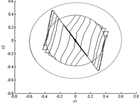
9] and [12]. 3 illustrate the origin, Theorem 2 for
tories and stabi
tories and stabi
included in th approximate tained from
elds to the f ith η=0.75
sible initial with
included in th approximately tained from
posed method ased up to 1.
th the ηmax o
the converge by using th two different
ility ball (η = 1.
ility ball (η = 0.
his ellipsoid is ly six times Theorem 2
feedback gain 5 , and the conditions is
(60)
his ellipsoid is y nine times Theorem 2
ds maximum 052 which is obtained from
ence of state he controller values of η.
.05 sec). .75 sec). s s 2 n e s s s 2 m s m e r
The inner ellipse in Fig. 2 shows the estimate of the domain of attractions. The outer ellipse in Fig. 3 shows the ellipsoid x PxT ≤β−1, as seen all trajectories begin
on the periphery of the inner ellipse never leave the outer ellipsoid and end up at the origin. Figs. 2 and 3 together with the information in Table 1 clarify that there is inverse relation between η and δmax.
6 Conclusion
In this paper two less conservative criteria have been presented to synthesis stabilizing controller for networked control system subject to input saturation. In the first method, the saturated linear system has been represented with a set of linear systems embedded within a convex polytope. In the second method, actuator saturation has been tackled via a generalized sector condition. Furthermore, an estimate of domain of attraction has been obtained through the LMI optimization. Illustrative example demonstrates the outperformance of the suggested methods compared to the existing approaches in the literature.
References
[1] A. Fereidunian, H. Lesani, C. Lucas, M. Lehtonen and M. M. Nordman, “A System Approach to Information Technology Infrastructure Design for Utility Management Automation Systems”, Iranian Journal of Electrical and Electronic Engineering, Vol. 2, No. 3, pp. 91-104, 2006. [2] C. Peng, Y.-C. Tian and M. O. Tade, “State
Feedback Controller Design of Networked Control Systems with Interval Time-varying Delay and Nonlinearity”, Int. Journal of Robust and Nonlinear Control, Vol. 18, No. 12, pp. 1285-1301, 2008.
[3] B. Tang, G.-P. Liu and W.-H. Gui, “Improvement of State Feedback Controller Design for Networked Control Systems”, IEEE Trans. on Circuits Systems II, Express Briefs, Vol. 55, No. 5, pp. 464-468, 2008.
[4] R. A. Gupta and M-Y. Chow, “Networked Control System, Overview and Research Trends”, IEEE Transactions on Industrial Electronics, Vol. 57, No. 7, pp. 2527-2535, 2010.
[5] M. Maboodi, M. H. Ashtari Larki and M. Aliyari Shoorehdeli, “An Under Load Servo Actuator Identification and Comparison between the Results of Different Methods”, Iranian Journal of Electrical and Electronics Engineering, Vol. 8, No. 3, pp. 227-233, 2012.
[6] A. Seuret and J. M. Gomes da Silva Jr., “Networked Control: Taking into Account Sample Period Variations and Actuator Saturation”, Proceeding of the 18th IFAC World Congress, pp. 1-6, 2011.
[7] Z. Xiaomeri, T. Hangji and L. Guoping, “Stabilization of Networked Stochastic Systems
Subject to Actuator Saturation”, Proceedings of 26th Chinese Control Conference, pp. 33-37, 2007.
[8] Z. Zuo, Y. Wang and G. Zhang, “Stability Analysis and Controller Design for Linear TimeDelay Systems with Actuator Saturation”, Proceedings of the 2007 American Control Conference, pp. 5840-5844, 2007.
[9] AE. Fridman, A. Seuret and J-P Richard, “Robust Sampled-data Stabilization of Linear Systems: an Input Delay Approach”, Automatica, Vol. 40, No. 8, pp. 1441-1446, 2004.
[10] E. Fridman, A. Pila and U. Shaked, “Regional Stabilization and H∞ Control of Time Delay systems with saturating actuators”, International Journal of Robust and Nonlinear Control, Vol. 13, No. 9, pp. 885-907, 2003.
[11] E. Fridman, “A Refined Input Delay Approach to Sampled-data Control”, Automatica, Vol. 46, No. 2, pp. 421-427, 2011.
[12] A. Seuret and J. M. Gomes da Silva Jr., “Taking into Account Period Variations and Actuator Saturation in Sampled-data Systems”, Systems and Control Letters, Vol. 61, No. 12, pp. 1286-1293, 2012.
[13] J. M. Gomes da Silva Jr., A. Seuret, E. Fridman and J. P. Richard, “Stabilization of Neutral Systems with Saturating Control Inputs” Int. Journal of Systems Science, Vol. 42, No. 7 , pp. 1093-1103, 2011.
[14] Z. Zuo, D. W. C. Ho, Y. Wang and C. Yang, “A New Approach for Estimating the Domain of Attraction for Linear Systems with Time-varying Delay and Saturating Actuators”, Proceedings of Seventh Asian Control Conference, pp. 274-279, 2009.
[15] J. M. Gomes da Silva Jr. and S. Tarbouriech, “Anti-windup Design with Guaranteed Regions of Stability for Discrete-time Linear Systems”, Systems and Control Letters, Vol. 55, No. 3, pp. 184-192, 2006.
[16] J. Sun, G. P. Liu, J. Chen and D. Rees, “Improved Stability Criteria for Linear Systems with Time Varying Delay”, IET Control Theory and Application, Vol. 4, No. 4, pp. 683-689, 2010. [17] T. Hu, Z. Lin and B. M. Chen, “An Analysis and
Design Method for Linear Systems Subject to Actuator Saturation and Disturbance”, Automatica, Vol. 38, No. 2, pp. 351-359, 2002. [18] S. Tarbouriech, J. M. Gomes da Silva Jr. and G.
Garcia, “Delay-dependent Anti-windup Strategy for Systems with Saturating and Delayed Outputs”, International Journal of Robust and Nonlinear Control, Vol. 14, No. 7, pp. 665–682, 2004.
Masod Mahmodi Kaleybar received his B.Sc. degree from Islamic Azad University of Tabriz, Tabriz, Iran, in 2008, and M.Sc. degree from Sahand University of Technology, Tabriz, Iran, in 2011, both in Electrical Engineering. His current research interests are analysis and design of networked control system.
Reza Mahboobi Esfanjani received his B.Sc. degree from Department of Electrical Engineering, Sahand University of Technology, Tabriz, Iran in 2002; He received the M.Sc. and Ph.D. degrees from Amirkabir University of Technology (Tehran Polytechnic) in 2004 and 2009, respectively. He has held faculty position at the Electrical Engineering Department, Sahand University of Technology, since 2010. His research interests include analysis and control of time-delay and networked systems.