R E S E A R C H A R T I C L E
Open Access
The competition between Lorentz and
Coriolis forces in planetary dynamos
Krista M. Soderlund
1*, Andrey Sheyko
2, Eric M. King
3and Jonathan M. Aurnou
4Abstract
Fluid motions within planetary cores generate magnetic fields through dynamo action. These core processes are driven by thermo-compositional convection subject to the competing influences of rotation, which tends to organize the flow into axial columns, and the Lorentz force, which tends to inhibit the relative movement of the magnetic field and the fluid. It is often argued that these forces are predominant and approximately equal in planetary cores; we test this hypothesis using a suite of numerical geodynamo models to calculate the Lorentz to Coriolis force ratio directly. Our results show that this ratio can be estimated by∗diRm−1/2(iis the traditionally defined Elsasser number
for imposed magnetic fields andRmis the system-scale ratio of magnetic induction to magnetic diffusion). Best estimates of core flow speeds and magnetic field strengths predict the geodynamo to be in magnetostrophic balance where the Lorentz and Coriolis forces are comparable. The Lorentz force may also be significant, i.e., within an order of magnitude of the Coriolis force, in the Jovian interior. In contrast, the Lorentz force is likely to be relatively weak in the cores of Saturn, Uranus, Neptune, Ganymede, and Mercury.
Keywords: Planetary dynamos; Core convection; Magnetic fields; Rotation; Magnetostrophic force balance
Background
Magnetic fields are common throughout the solar sys-tem and provide a unique perspective on the internal dynamics of planetary interiors. Planetary magnetic fields are driven by the conversion of kinetic energy into mag-netic energy; this process is called dynamo action. Kimag-netic energy is derived from thermo-compositional convection of an electrically conducting fluid although mechanical mechanisms, such as libration and precession, may also drive core flow in smaller bodies (e.g., Le Bars et al. 2015). The geodynamo is the most studied planetary mag-netic field, yet the mechanisms that control its strength, morphology, and secular variation are still not well under-stood. Towards explaining these observations, dimension-less parameters are often used to characterize the force balances present in the core and their link to processes that govern convective dynamics and dynamo action. Two forces that are particularly influential on core processes are the Coriolis force, which tends to organize the core
*Correspondence: [email protected]
1Institute for Geophysics, John A. & Katherine G. Jackson School of Geosciences, The University of Texas at Austin, J. J. Pickle Research Campus, Building 196 (ROC), 10100 Burnet Road (R2200), Austin, Texas, 78758-4445, USA Full list of author information is available at the end of the article
fluid motions, and the Lorentz force which back-reacts on the fluid motions to equilibrate magnetic field growth.
In order to better understand the manifestation of Coriolis and Lorentz forces on core flow, let us consider the Boussinesq momentum equation. In this commonly used approximation, the material properties are assumed to be constant and the density is treated as constant except in the buoyancy force of the momentum equation (e.g., Tritton 1998):
Du
Dt +2×u= −∇−αT
g+ν∇2u+ 1
ρo
J×B. (1)
of the motionless background state (assumed to be con-stant densityρo). These perturbations,ρ/ρo= −αT, are produced by temperature variations, T, from the back-ground state temperature profile;αis thermal expansivity. Viscous diffusion depends on the kinematic viscosity of the fluid, ν. The Lorentz force is due to interactions between the magnetic field and current density.
Planetary cores are rapidly rotating and the Coriolis force is expected to be large compared to the viscous, iner-tial, and buoyancy forces at global scales (the former two forces are scale dependent quantities). If we neglect these forces and magnetic fields in the Boussinesq momentum equation (Eq. 1), the system is in geostrophic balance:
2×u= −∇. (2)
This balance requires horizontal fluid motions to fol-low lines of constant pressure. Further insight can be obtained by taking the curl of Eq. 2 and using the continu-ity equation (∇ ·u=0) to obtain· ∇u=0. If we assume =zˆwhereis constant, this equation simplifies to
∂u
∂z =0. (3)
This is the Taylor-Proudman theorem and states that the fluid motion will be invariant along the direction of the rotation axis. However, in order for convection to occur, the Taylor-Proudman constraint cannot strictly hold as there must be slight deviations from two-dimensionality, at least in the boundary layers, to allow overturning motions in the fluid layer (e.g., Zhang 1992; Olson et al. 1999; Grooms et al. 2010). Further beyond the onset of convection, convective flows break down into an anisotropic rotating turbulence (e.g., Sprague et al. 2006; Julien et al. 2012; Stellmach et al. 2014; Cheng et al. 2015; Ribeiro et al. 2015).
Linear asymptotic analyses of quasigeostrophic con-vection predict that the azimuthal wavenumber of these columns relative to the thickness of the fluid shell varies as
U/D∝E1/3, where the Ekman number,E=ν/
2D2, represents the ratio of viscous to Coriolis forces (e.g., Roberts 1968; Julien et al. 1998; Jones et al. 2000; Dormy et al. 2004). Thus, in rapidly rotating systems such as plan-etary cores (whereE 10−12), it is often predicted that quasigeostrophic convection occurs as tall, thin columns (e.g., Kageyama et al. 2008; cf. Cheng et al. 2015).
In planetary dynamos, however, magnetic fields are also thought to play an important dynamical role on the con-vection and zonal flows. When strong imposed magnetic fields and rapid rotation are both present, the dominant force balance is magnetostrophic—a balance between the Coriolis, pressure gradient, and Lorentz terms:
2×u= −∇+ 1
ρo
J×B. (4)
In contrast to Eq. 3, the curl of the magnetostrophic balance Eq. 4 yields
∂u
∂z = −
1
2ρo∇ ×(
J×B). (5)
This equation shows that magnetic fields can relax the Taylor-Proudman constraint, allowing global-scale motions that differ fundamentally from the small-scale axial columns typical of non-magnetic, rapidly rotat-ing convection (e.g., Cardin and Olson 1995; Olson and Glatzmaier 1996; Zhang and Schubert 2000; Roberts and King 2013).
Magnetic fields are typically considered to be important dynamically when the ratio of Lorentz to Coriolis forces is of order unity. This ratio is represented by the Elsasser number, , which can be approximated by assuming a characteristic current density, magnetic induction, den-sity, rotation rate, and velocity scale:
= Lorentz Coriolis=
1
ρoJ×B
|2×u| ≈ JB 2ρoU
. (6)
In systems where the magnetic field is not strongly time variant (i.e., ∂B/∂t = −∇ ×E ∼ 0), the current den-sity can be approximated via Ohm’s Law,J∼σUBwhere
σ = (μoη)−1is electrical conductivity andηis magnetic diffusivity, such that
i=
B2 2ρoμoη
. (7)
This formulation is thus appropriate for steady imposed magnetic fields (e.g., Olson and Glatzmaier 1996; King and Aurnou 2015). In dynamos, which tend to exhibit signifi-cant temporal variability, it is more appropriate to approx-imate the current density using Ampere’s law under the MHD approximation,J ∼ B/μo Bwhere B is the char-acteristic length scale of magnetic field variations (e.g., Cardin et al. 2002; Soderlund et al. 2012). In thisdynamic case, Eq. 6 becomes
d=
B2 2ρoμoU B =
i
Rm D
B
, (8)
indicating that the Lorentz to Coriolis force ratio is length scale dependent. In the latter equality,Rm=UD/ηis the global ratio of magnetic induction to magnetic diffusion. This parameter must exceed approximately 10 in order for dynamo action to occur (e.g., Roberts 2007). Thus, on global scales, where B D, the dynamic Elsasser number will always be less than i by at least an order of magnitude for active dynamos. However, the influence of magnetic fields will become increasingly important at smaller scales sinced∝ −1B in (Eq. 8).
be estimated from observations, such asiandRm. The length scale Bcan be approximated using the magnetic induction equation:
∂B
∂t = ∇ ×(u×B)+η∇
2B (9)
Assuming a balance between induction and diffusion yields UB/D ∼ ηB/ 2B. Rearranging, the dimensionless length scale is proportional to the inverse square root of the magnetic Reynolds number:
B/D∼Rm−1/2 (10)
(e.g., Galloway 1978; King and Roberts 2013). Using this relationship in Eq. 8, we estimate the dynamic Lorentz to Coriolis force ratio to be
∗d∼iRm−1/2. (11)
This scaling estimate will be referred to as themodified dynamicElsasser number.
In this paper, we will investigate the relative magnitudes of Lorentz and Coriolis forces to better understand the dynamics of planetary cores. Towards this end, we calcu-late directly the Lorentz to Coriolis force ratio in a suite of geodynamo models described in the “Methods” section, test Eq. 11 to predict this ratio in the “Results” section, and extrapolate the results to Earth and other planetary cores in the “Discussion” section.
Methods
We analyze 34 dynamo models presented in Soderlund et al. (2012, 2014) and five dynamo models presented in Sheyko (2014); these datasets will be referred to as SKA and S14, respectively. These simulations of Boussinesq convection and dynamo action are carried out in thick, rotating spherical shells with thicknessD, rotation rate, and no-slip boundaries. Gravity is assumed to vary lin-early with radius;gois acceleration at the top of the fluid shell. The outer boundary at radiusrois assumed electri-cally insulating and the solid inner core at radiusri has the same electrical conductivity as the convecting fluid region.
The SKA dataset considers three rotation rates (Ekman numbers in the range 10−3 ≥ E ≥ 10−5), two magnetic diffusivities (magnetic Prandtl numbers ofPm = 2, 5), and thermal forcing near onset (Rac) to more than 1000 times critical (1.9<Ra/Rac< 1125); the shell geometry is fixed toχ = ri/ro = 0.4 with isothermal boundaries. This survey is complemented by the S14 dataset focusing on low Ekman, low magnetic Prandtl number simulations: 3×10⁻⁷ E 10−6, 0.05≤ Pm≤1, and 108 Ra 1010 with χ = 0.35, an isothermal inner shell bound-ary, and fixed heat flux on the outer shell boundary. For both datasets, the thermal (κ) and momentum (ν) diffu-sivities are assumed equal, such that the Prandtl number,
Pr=ν/κ, is unity. Here,E=ν/2D2is the ratio of vis-cous to Coriolis forces;Pm = ν/ηis the ratio of viscous to magnetic diffusivities, andRa=αgoTD3/(νκ)is the ratio of buoyancy due to superadiabatic temperature con-trastT to diffusion. The combination of these datasets, given in Table 1, results in one of the broadest surveys of supercriticality, Ekman, and magnetic Prandtl numbers in the literature.
The SKA simulations are carried out on numerical grids that range from 37 fluid shell radial levels and 42 spherical harmonic degrees (near onset atE = 10−3) to 73 radial levels and 213 spherical harmonic degrees (highestRafor E = 10−5). Hyperdiffusion is used for the three most extreme cases (Ra ≥ 2×10⁸forE ≤ 10−4); additional details are given in Soderlund et al. (2012). The S14 sim-ulations are carried out on numerical grids with 512–528 radial levels and 256 spherical harmonic degrees. All sim-ulations are carried out using pseudo-spectral methods with no azimuthal symmetries assumed (Wicht 2002; Christensen and Wicht, 2007; Sheyko 2014). Once the ini-tial transient has subsided, global diagnostic quantities (i,Rm, B,d, and∗d) are time-averaged to minimize statistical errors.
In our models, the imposed Elsasser number is calcu-lated from the dimensionless magnetic energy density,EM, within the fluid shell of volumeV:
i=2PmEEMwhereEM = 1 2Pm E V
V
B·BdV,
(12)
while the magnetic Reynolds number is calculated from the dimensionless kinetic energy density,EK:
Rm=2EKPmwhereEK = 1 2V
V
u·udV. (13)
These quantities are non-dimensionalized using distance, magnetic induction, velocity, and energy density scales of D=ro−ri,√2ρμoη,ν/D, andρν2/D2, respectively. We also characterize Bas a quarter wavelength of the typical magnetic field wavenumber (Soderlund et al. 2012):
B/D∼ (π/
2)
lB2+mB2
, where lB=
l(Bl·Bl) 2Pm EEM
and
mB=
m(Bm·Bm) 2Pm EEM
.
(14)
Here, Bl and Bm are magnetic induction at spherical harmonic degreeland orderm.
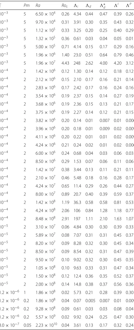
Table 1Input (E,Pm,Ra,Roc=
RaE2/Pr) and output (
i,d,
∗
d,I,P) parameters for our dataset.Pr=1 is fixed for all
simulations. Additional simulation information is given in Soderlund et al. (2012, 2014) for cases withE≥10−5and Sheyko
(2014) for cases withE10−6
E Pm Ra Roc i d ∗d I P
10−3 5 6.50×10⁴ 0.26 4.34 0.44 0.47 0.39 0.26
10−3 5 9.70×10⁴ 0.31 3.91 0.30 0.35 0.43 0.32
10−3 5 1.12×10⁵ 0.33 3.25 0.20 0.25 0.40 0.29
10−3 5 1.32×10⁵ 0.36 0.61 0.03 0.04 0.05 0.01
10−3 5 5.00×10⁵ 0.71 4.14 0.15 0.17 0.29 0.16
10−3 5 1.96×10⁶ 1.40 23.0 0.51 0.64 0.79 0.46
10−3 5 1.96×10⁷ 4.43 248 2.62 4.00 4.20 3.12
10−4 2 1.42×10⁶ 0.12 1.30 0.14 0.12 0.18 0.12
10−4 2 2.12×10⁶ 0.15 2.10 0.17 0.16 0.21 0.14
10−4 2 2.83×10⁶ 0.17 2.42 0.17 0.16 0.24 0.16
10−4 2 3.54×10⁶ 0.19 2.37 0.15 0.14 0.27 0.19
10−4 2 3.68×10⁶ 0.19 2.36 0.15 0.13 0.21 0.17
10−4 2 3.75×10⁶ 0.19 2.27 0.14 0.12 0.21 0.15
10−4 2 3.82×10⁶ 0.20 0.14 0.01 0.007 0.01 0.006
10−4 2 3.96×10⁶ 0.20 0.18 0.01 0.009 0.02 0.009
10−4 2 4.11×10⁶ 0.20 0.22 0.01 0.01 0.02 0.009
10−4 2 4.24×10⁶ 0.21 0.24 0.02 0.01 0.02 0.006
10−4 2 6.00×10⁶ 0.24 0.68 0.04 0.03 0.06 0.03
10−4 2 8.50×10⁶ 0.29 1.53 0.07 0.06 0.11 0.06
10−4 2 1.42×10⁷ 0.38 3.44 0.13 0.11 0.21 0.11
10−4 2 2.10×10⁷ 0.46 5.48 0.18 0.16 0.28 0.17
10−4 2 4.24×10⁷ 0.65 11.4 0.29 0.26 0.44 0.27
10−4 2 8.00×10⁷ 0.89 20.7 0.40 0.39 0.59 0.37
10−4 2 1.42×10⁸ 1.19 36.3 0.58 0.58 0.81 0.53
10−4 2 4.24×10⁸ 2.06 106 0.84 1.28 1.18 0.77
10−4 2 8.48×10⁸ 2.91 197 1.11 2.10 1.63 1.07
10−5 2 3.10×10⁷ 0.06 4.84 0.30 0.30 0.39 0.33
10−5 2 5.89×10⁷ 0.08 7.07 0.31 0.31 0.45 0.37
10−5 2 8.20×10⁷ 0.09 8.28 0.32 0.30 0.45 0.34
10−5 2 8.50×10⁷ 0.09 8.54 0.32 0.31 0.47 0.39
10−5 2 9.50×10⁷ 0.10 9.02 0.32 0.30 0.45 0.35
10−5 2 1.05×10⁸ 0.10 9.63 0.33 0.31 0.47 0.34
10−5 2 1.50×10⁸ 0.12 12.4 0.36 0.35 0.52 0.37
10−5 2 2.00×10⁸ 0.14 14.8 0.38 0.37 0.56 0.36
1.2×10⁻⁶ 1 1.86×10⁸ 0.02 5.73 0.21 0.28 0.39 0.30 1.2×10⁻⁶ 0.2 1.86×10⁸ 0.04 0.07 0.005 0.007 0.01 0.009 1.2×10⁻⁶ 0.2 9.28×10⁸ 0.09 0.61 0.03 0.03 0.08 0.04 1.2×10⁻⁶ 0.2 5.57×10⁹ 0.02 9.92 0.24 0.25 0.47 0.30
3.0×10⁻⁷ 0.05 2.23×10¹⁰ 0.04 3.61 0.13 0.17 0.32 0.24
(FL) and Coriolis (FC) forces over the spherical shell
vol-ume following Soderlund et al. (2012):
FLI =
V
FL· ˆr
2+ FL· ˆθ
2
+FL· ˆφ
21/2
dV (15)
FCI =
V
FC· ˆr
2
+FC· ˆθ
2
+FC· ˆφ
21/2
dV (16)
where the volume-integratedforce ratio isI = FLI/FCI. Alternatively, the root mean square (RMS) Lorentz and Coriolis forces are calculated at each grid point to deter-mine the force ratio locally (cf. Dharmaraj and Stanley 2012; Dharmaraj et al. 2014). A representative value is determined by taking the most probable ratio in the histogram; this probability approach yields P (Fig. 1). Histogram bins are uniformly spaced to contain equal ranges of log10
FLRMS/FCRMS values. The probability of each bin is defined as the volume of the fluid shell that is occupied by the respective range of force ratio values relative to the total volume of the fluid shell. For both approaches, velocity and magnetic fields from three ran-dom snapshots in time are used to calculate the force ratios for the SKA dataset, with I and P being the average values. Single snapshots are used for the S14 dataset.
Results
A Lorentz to Coriolis force ratio histogram is evaluated for a representative dipole-dominated dynamo case at a snap-shot in time in Fig. 1. The histogram indicates that the
0 0.2 0.4 0.6 0.8 1.0 1.2 1.4 1.6 1.8 2.0
-3 -2 -1 0 1 2 3
0 0.005 0.010 0.015 0.020 0.025 0.030 0.035
Log10 Lorentz/Coriolis Forces 0.040
ΛP
Fraction of Shell V
olume
-4
0.045 Mean Kinetic Energy of Bin / Mean Kinetic Energy
Coriolis force is dominant for the majority of grid points, most frequently by an order of magnitude. Moreover, the points with Lorentz to Coriolis force ratios greater than unity tend to have relatively low kinetic energies, denoted by coloration of the bins. Thus, the Lorentz force is expected to have a secondary influence on the convective (non-zonal) dynamics (Soderlund et al. 2012). This does not mean, however, that the magnetic field cannot have an important, local-scale dynamical impact (cf. Sreenivasan and Jones 2011).
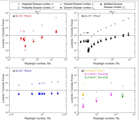
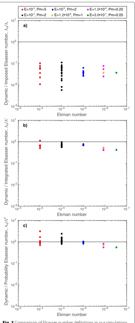
Figure 2 shows the ratio of Lorentz to Coriolis forces in our simulations as characterized by theintegratedI, probability P, imposed i, dynamic d, and modified dynamic∗dElsasser numbers (see Table 2 for a summary
of definitions). For comparison, ratios of these parame-ters are plotted in Fig. 3. Thei Elsasser number, which is traditionally used to test for magnetostrophic balance, substantially overestimates the Lorentz to Coriolis force ratio in all of our dynamo models (i.e., typically by an order of magnitude; see Fig. 3a). In contrast, we find that all of the other Lorentz to Coriolis force ratio definitions (I,
P,
d, ∗d) agree to within a factor of five; a factor of 1.4 is the mean deviation between definitions. Comparing the in situ calculations,IexceedsPin all cases investi-gated. This result implies that, independent of the Ekman and magnetic Prandtl numbers and in agreement with the literature (e.g., Aubert et al. 2008, Sreenivasan et al. 2014), the Lorentz force is concentrated in discrete regions that
104 105 106 107 108
Rayleigh number, Ra a)E=10-3, Pm=5
10
107 108
106 109
Rayleigh number, Ra
Lorentz / Coriolis Force
b) E=10-4, Pm=2
1010
Rayleigh number, Ra
Lorentz / Coriolis Force
d)
-3
10-2
10-1
100
3
10 10
1011
108
108
Rayleigh number, Ra
Lorentz / Coriolis Force
c) E=10-5, Pm=2
3.108
2.107 109
101
102
-3
10-2
10-1
100
3
10 10
101
102
-3
10-2
10-1
100
3
10 10
101
102
-3
10-2
10-1
100
3 10
101
102
Integrated Elsasser number,ΛI
Probability Elsasser number,ΛP Dynamic Elsasser number,Λ d
Modified Dynamic Elsasser number, Λd Imposed Elsasser number,Λi
E=1.2•10-6, Pm=1
E=1.2•10-6, Pm=0.20
E=3.0•10-7, Pm=0.05
Lorentz / Coriolis Force
*
Roc=1 Roc=1
Fig. 2 a–dDirect calculations and parameterizations of the Lorentz to Coriolis force ratio in our simulations. Lorentz to Coriolis force ratios as a function of Rayleigh number for five Ekman numbers and five magnetic Prandtl numbers. The modified dynamic Elsasser number includes the length scale pre-factor:∗d=0.77iRm−1/2. The Rayleigh numbers corresponding toRo
c=
Table 2Elsasser number definitions: (1) Imposedi, (2) Dynamic
d, (3) Modified dynamic∗d, (4) IntegratedI, and (5)
ProbabilityP
i d ∗
d I P
B2
2ρoμoη
i
RmDB 0.77
i
Rm1/2
V|FL|dV
V|FC|dV
|FL|
|FC|, max probability
are more influenced by magnetic fields than the rest of the fluid volume. Similarly, the dynamic Elsasser num-ber is also found to be in better agreement withPthan
I(Fig. 3b, c); the mean (maximum) percent differences betweendandP are 28 % (68 %) forE = 10−3, 18 % (58 %) forE = 10−4, 9 % (21 %) forE = 10−5, and 49 % (80 %) forE10−5.
The Lorentz to Coriolis force ratios in Fig. 2 have dis-tinct minima for cases withE ≥ 10−4. This sharp drop as the Rayleigh number is increased from onset occurs when the dipole-dominance of the dynamo breaks down. The Lorentz force increases more rapidly than the Coriolis force asRais further increased (see Fig. 4a of Soderlund et al. 2012), which explains the subsequent increase in Elsasser numbers.
Before discussing the modified Elsasser number, the assumption that the dimensionless length scale represen-tative of magnetic field gradients in our simulations is approximately equal to the theoretical prediction (Eq. 10) must be assessed. This comparison is made in Fig. 4. Agreement within a factor of two—and typically much less, 16 % difference on average—between the B/Dvalues calculated directly from our simulations and the scal-ing estimate occurs when a pre-factor of 1.3 is included in Eq. 10:
B/D=1.3Rm−1/2. (17)
This pre-factor is determined by minimizing the least squares residual between the calculated and predicted values across our dataset. Roberts and King (2013) also investigated the length scale of magnetic field varia-tions in geodynamo models and found a similar depen-dence on Rm−1/2 with a pre-factor of 3 due to their slightly modified definition of B/D. More importantly, they also show that the magnetic length scale is weakly dependent on the magnetic field strength i, which may explain some of the spread in our model-prediction deviations.
The modified dynamic Elsasser number is given by solid, starred markers in Fig. 2; here, ∗d has been modified compared to Eq. 11 to include the pre-factor derived from the length scale calculations (Eq. 17):
∗
d=0.77iRm−1/2. (18)
For all Ekman numbers, the dynamic d and modified dynamic∗d Elsasser numbers differ by less than a factor
Ekman number
10-2 10-3 10-4 10-5 10-6 10-7
Dynamic / Imposed Elsasser number,
Λd
/
Λi
10-3
10-2
10-1
100
101
Ekman number
10-2 10-3 10-4 10-5 10-6 10-7
Dynamic / Integrated Elsasser number,
Λd
/
Λ
I
10-3
10-2
10-1
100
101
a)
b)
Ekman number
10-2 10-3 10-4 10-5 10-6 10-7
Dynamic / Probability Elsasser number,
Λd
/
Λ
P
10-3
10-2
10-1
100
101
c)
E=10-3, Pm=5
E=10-4, Pm=2
E=10-5, Pm=2 E=1.2•10-6, Pm=0.20
E=3.0•10-7, Pm=0.05
E=1.2•10-6, Pm=1
Fig. 3Comparison of Elsasser number definitions in our simulations. Ratio of the dynamic Elsasser numberdto theaimposed Elsasser numberi,bintegrated Elsasser numberI, andcprobability Elsasser numberPas a function of Ekman number
E 10−6. The differences between ∗d and the proba-bility Elsasser numberP tend to be comparable: 28 % (73 %) forE = 10−3, 16 % (49 %) forE = 10−4, 13 % (28 %) forE=10−5, and 25 % (43 %) forE10−6. Thus, the modified dynamic Elsasser number∗daccurately cap-tures the ratio of Lorentz to Coriolis forces in our suite of simulations.
In order to apply the modified dynamic Elsasser number to planetary cores, its applicability to core conditions must first be evaluated. Our datasets cover a broad range of diagnostic physical parameters: magnetic field strengths of 10−1 i 102, magnetic induction to diffusion ratios of 102 Rm 104, and Lorentz to Coriolis force ratios of 10−2 d 1. However, these ranges span only a fraction of the planetary parameter estimates, which vary over 10−5 i 1010, 102 Rm 105, and 10−6 ∗d 107as detailed in the “Discussion” section. The most fundamental deviation is ford > 1, which implies a different dominant force balance. While our dataset includes cases withd>1, these simulations are strongly driven with inertia exceeding both Lorentz and Coriolis forces (see Fig. 4 of Soderlund et al. 2012), which is not expected for most planets (cf. Soderlund et al. 2013).
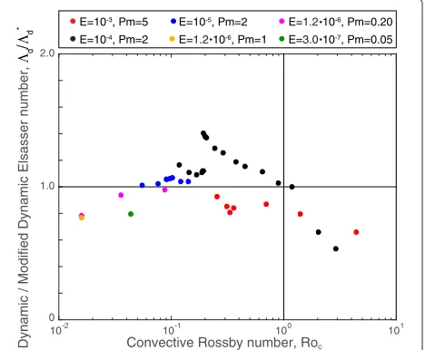
Figure 5 shows the ratio of the dynamic to modified dynamic Elsasser numbers as a function of the convective Rossby number,Roc=
RaE2/Pr1/2, which characterizes the ratio of buoyancy-driven inertial forces to Coriolis forces (e.g., Gilman 1977, Aurnou et al. 2007). The ∗d approximation works well when the Coriolis force dom-inates; in contrast, the largest discrepancy occurs when Roc > 1. Geodynamo simulations from Dormy (2014) provide a∗d test for cases withd > 1 and Roc < 1 at an Ekman number ofE = 1.5×10⁻⁴and a Prandtl number of unity. Here, large magnetic Prandtl num-bers (Pm ≥ 12) are required to obtain dynamo action since the inertial forces are relatively weak (i.e., quasi-laminar flows). Application of Eq. 18 to his dataset yields 0.85 ≤ d/∗d ≤ 1.3, implying that our results are applicable to strong field systems with dominant Lorentz forces.
A discrepancy between input parameters also exists between the simulations and planetary cores. In particu-lar, all numerical dynamo models are necessarily limited to massively overestimated kinematic viscosities, which prohibits simulations with realistic Ekman and magnetic Prandtl numbers: 10−19 E 10−12and 10−8 Pm 10−6are estimated for planets with active dynamos (e.g., Schubert and Soderlund 2011). In contrast, our dataset considers 10−7 E 10−3 and 10−1 Pm 101. Importantly, no clear Ekman or magnetic Prandtl number dependence is identified in Fig. 5. We, therefore, hypoth-esize that the modified dynamic Elsasser number (Eq. 18) can be extrapolated to extreme planetary parameters.
1012
Solid: calculated Hollow: predicted
106 108
104 1010
Rayleigh number, Ra
Magnetic Length Scale,
B
/D
0.0
107 109
105 1011 0.1
0.2
E=10-3, Pm=5
E=10-4, Pm=2
E=10-5, Pm=2 E= 10-6, Pm=0.20
E= 10-7, Pm=0.05
E=
1.2 3.0 1.210-6, Pm=1
Fig. 4Calculated and predicted magnetic length scales. Magnetic length scale as a function of the Rayleigh number with Ekman and magnetic Prandtl numbers denoted bycolor. A best-fit between the calculated and predicted values is obtained when a pre-factor is included in (Eq. 10): B/D=1.3Rm−1/2(included here)
Discussion
The modified dynamic Elsasser number can be used to estimate the Lorentz to Coriolis force ratio in planetary cores wheniandRmare known (see Fig. 6 and Table 3). The imposed Elsasser number is traditionally used to quantify magnetic field strengths of planets since the poloidal component (Bp) can be measured by spacecraft and estimates for the other components (densityρ, mag-netic diffusivity η, and rotation rate ) are relatively
Convective Rossby number, Roc
10-2 10-1 100 101
Dynamic / Modified Dynamic Elsasser number,
Λd
/
Λd
*
0 1.0 2.0
E=10-3, Pm=5
E=10-4, Pm=2
E=10-5, Pm=2 E=1.210-6, Pm=0.20
E=3.010-7, Pm=0.05
E=1.210-6, Pm=1
Fig. 5Comparison of predicted and calculated Elsasser numbers as a function of the relative strengths of buoyancy and Coriolis forces. Ratio ofd/∗dplotted versus the convective Rossby number, Roc=
2 1
2 3 4 5 6
Imposed Elsasser number, Λi
Magnetic Reynolds number
, Rm
10 104 108
-4
10
-6
10 10 10 10 10 10 10
-6 -4 -2 2 4 6
10 10 10 10 10 10 Modified Dynamic Elsasser number,
Λ
d
Λd= 1
0
10
Earth Jupiter
Ice Giants Saturn
Mercury Ganymede
-2
10 100 106 1010
*
*
Fig. 6Lorentz to Coriolis force ratio predictions for planetary cores. Modified dynamic Elsasser number as a function of imposed Elsasser number and magnetic Reynolds number across a range of values that may be relevant to planets in our solar system as well as exoplanets. The approximate ranges of anticipatediandRmvalues are given for planets with active dynamos.Barred line endsforidenote the observed magnetic field strengths;arrowed line endsdenote upper bounds.Barred line endsforRmdenote constrained bounds;arrowed line endsdenote a larger range of uncertainties. Black circles denote the most probableiandRmvalues
straightforward (see Schubert and Soderlund 2011 for a review); these measurements constitute a lower bound since the toroidal component is not included and small-scale poloidal contributions are below the resolution of detection. Toroidal magnetic fields (BT) can be amplified by stretching of the poloidal field due to azimuthal dif-ferential rotation (zonal flows). This so-called ω-effect can generate toroidal magnetic fields up toBT ∼ RmBp (Roberts 2007), which sets an i upper bound. For a best estimate, we assume the total core field strengthB to be an order of magnitude larger than the direct mea-surements (i.e., i increases by a factor of 100). This assumption is motivated both by geomagnetic data (e.g., Shimizu et al. 1998) and geodynamo modeling results (e.g., Aubert et al. 2009).
Earth:Geodynamo core flow inversions based on sec-ular variation of the magnetic field imply velocities of U∼5×10⁻⁴m/s (e.g., Holme 2007; Aubert 2013), which corresponds toRm∼103assumingη∼1 m2/s for liquid
Table 3Order of magnitude estimates of the magnetic Reynolds
numberRm, the imposed Elsasser numberi, and the Lorentz to
Coriolis force ratio as estimated by∗dfor planetary cores with active dynamos
Mercury Earth Ganymede Jupiter Saturn Ice Giants
Rm 75 103 500 105 104 102
i 10−3 102 10−1 102 100 10−2
∗
d 10−4 100 10−3 10−1 10−2 10−3
metals. Ensemble inversions further suggest RMS mag-netic field strengths in the cylindrical direction ofBS ∼2 mT (Gillet et al. 2010), while toroidal magnetic field con-straints of 1 < BT/BS < 100 have been inferred by Shimizu et al (1998). Thus,B∼10BS∼20 mT appears to be a reasonable estimate of the core’s total field strength such that i ∼ 102. In contrast, direct magnetic field measurements suggest a lower bound ofi∼1 and appli-cation of the ω-effect suggests an upper bound ofi ∼ 106. We, therefore, predict a Lorentz to Coriolis force ratio of∗d ∼ 1 for the geodynamo, with a possible range of 10−2 ∗d 104. This result suggests that the Lorentz force cannot be neglected dynamically in the core and, more likely, that the core is in magnetostrophic balance.
i ∼ 10−5and∼ 10−1for Mercury, which corresponds to∗d 10−2and implies that magnetostrophic balance is unlikely in the Hermian core. Conversely, the possible magnetic field strengths for Ganymede range fromi ∼ 10−3to∼102, yielding 10−5∗
d1. However, the best estimate for the imposed Elsasser number isi ∼ 10−1 such that ∗d ∼ 10−3. As a result, magnetostrophic balance is possible, but unlikely, in Ganymede’s core.
Gas Giants:Jovian velocities can be estimated through scaling arguments and potentially secular variation. Jones (2014) suggests flow velocities ofU 10−3m/s, leading to values ofRm 105 given the planet’s large size. In this case, magnetic field strengths range from i ∼ 1 via core field measurements toi ∼ 1010 when theω -effect is included, with a best estimate ofi ∼ 102. The corresponding Lorentz to Coriolis force ratio then spans the range 10−3 ∗d 107, with∗
d ∼ 0.1 being the best estimate. Thus, barring the large uncertainties, the Lorentz force is predicted to be sub-dominant, but not negligible, in Jupiter’s core.
Starchenko and Jones (2002) predict similar flow speeds for the Saturnian interior, which corresponds to a lower Rm ∼ 104 value due to the smaller size of the dynamo region. Saturn’s magnetic field is also weaker than that of Jupiter; the best estimate imposed Elsasser number is
i ∼ 1 with a feasible range of 10−2 i 106. In the most likely scenario, the Lorentz force is predicted to be two orders of magnitude smaller than the Coriolis force (∗d ∼ 10−2) with uncertainties extending the possible range to 10−4∗d104.
Ice Giants: Uranus and Neptune have relatively weak core magnetic fields with i ∼ 10−4 based on space-craft observations, but there are few constraints on the flow speeds. We, therefore, assumeU ∼ 10−3m/s based on the other planetary estimates such thatRm ∼ 102to give an upper bound ofi ∼ 1 when the toroidal esti-mate is included. For these i estimates, the predicted Lorentz to Coriolis force ratio is always less than unity: 10−5 ∗d 10−1. These results thus imply that the ice giants are not in magnetostrophic balance.
Conclusions
The Lorentz to Coriolis force ratio is an important parameter for the dynamics of planetary cores since dynamos with dominant Coriolis forces at global scales are expected to be driven by fundamentally different archetypes of fluid motions than those with dominant (or co-dominant) Lorentz forces (Roberts and King 2013, Calkins et al. 2015). We hypothesize that a representa-tive global estimate of the Lorentz to Coriolis force ratio can be predicted by∗d = 0.77iRm−1/2. An advantage of this formulation is that it depends on quantities that can be estimated for planetary cores (Table 3). Our results
suggest that the Earth’s core is likely to be in magne-tostrophic balance where the Lorentz and Coriolis forces are comparable. The Lorentz force may also be substan-tial in Jupiter’s core, where it is predicted to be a factor of ten less than the Coriolis force. Magnetic fields become increasingly sub-dominant for the other planets: the Cori-olis force is predicted to exceed the Lorentz force by at least two orders of magnitude within the cores of Saturn, Uranus/Neptune, Ganymede, and Mercury.
These conclusions are subject to large uncertainties, however. Core flow speeds are difficult to estimate, while total magnetic field strengths cannot be measured directly. The applicability of Eq. 18 for the Lorentz to Coriolis force ratio may also break down at extreme plan-etary core conditions that cannot be explored numerically or in the laboratory due to technological limitations. In order to mitigate these uncertainties, we have considered a range of possible core magnetic field strengths (i) and included state-of-the-art simulations (Sheyko 2014; cf. Nataf and Schraeffer 2015).
Abbreviations
MHD: Magnetohydrodynamics; RMS: Root mean square; SKA: Soderlund et al. (2012, 2014); S14: Sheyko 2014.
Competing interests
The authors declare that they have no competing interests.
Authors’ contributions
KMS and JMA designed the study. KMS and AS carried out and analyzed the numerical simulations. All authors interpreted the data. All authors read and approved the final manuscript.
Acknowledgements
The authors thank two anonymous referees for their thoughtful reviews, Hao Cao for helpful suggestions, and Wolfgang Bangerth for enlightening discussions at the 2014 Study of Earth’s Deep Interior (SEDI) meeting in Kanagawa, Japan. KMS gratefully acknowledges Japan Geoscience Union the National Science Foundation to attend this symposium as well as research support from the National Science Foundation (grant AST-0909206). JMA acknowledges the support of the National Science Foundation Geophysics Program (grant EAR-1246861). Computational resources supporting this work were provided by the NASA High-End Computing (HEC) Program through the NASA Advanced Supercomputing (NAS) Division at Ames Research Center and by the Swiss National Supercomputing Centre (CSCS) under project ID s225. This is UTIG contribution 2858.
Author details
1Institute for Geophysics, John A. & Katherine G. Jackson School of
Geosciences, The University of Texas at Austin, J. J. Pickle Research Campus, Building 196 (ROC), 10100 Burnet Road (R2200), Austin, Texas, 78758-4445, USA.2Institut für Geophysik, ETH Zürich, NO H 11.2, Sonneggstrasse 5 8092 Zürich, LA59 Switzerland.3U.S. Global Development Lab, U.S. Agency for
International Development, Washington, DC, 20004, USA.4Department of Earth, Planetary, and Space Sciences, University of California, Los Angeles, 595 Charles Young Drive East, Los Angeles, California, 90095-1567, USA.
Received: 1 April 2015 Accepted: 10 August 2015
References
Aubert J, Labrosse S, Poitou C (2009) Modelling the palaeo-evolution of the geodynamo. Geophys J Int 179:1414–1428
Aubert J (2013) Flow throughout the Earth’s core inverted from geomagnetic observations and numerical dynamo models. Geophys J Int 192:537–556 Aurnou JM, Heimpel MH, Wicht J (2007) The effects of vigorous mixing in a
convective model of zonal flow on the Ice Giants. Icarus 190:110–126 Calkins MA, Julien K, Tobias SM, Aurnou JM (2015) A multiscale dynamo model
driven by quasi-geostrophic convection. J Fluid Mech. doi:10.1017/jfm.2015.464
Cao H, Aurnou JM, Wicht J, Dietrich W, Soderlund KM, Russell CT (2014) A dynamo explanation for Mercury’s anomalous magnetic field. Geophys Res Lett 41(12):4127–4134
Cardin P, Olson PL (1995) The influence of toroidal magnetic field on thermal convection in the core. Earth Planet Sci Lett 133:167–181
Cardin P, Brito D, Jault D, Nataf HC, Masson JP (2002) Towards a rapidly rotating liquid sodium dynamo experiment. Magnetohydrodynamics 38:177–189 Cheng JS, Stellmach S, Ribeiro A, Grannon A, King EM, Aurnou JM (2015)
Laboratory-numerical models of rapidly rotating convection in planetary cores. Geophys J Int 201:1–17
Christensen U. R, Wicht J (2007) Numerical Dynamo Simulations. In: Schubert G (ed). Treatise on Geophysics, Core Dynamics. Elsevier, Amsterdam Vol. 8. pp 245–282. Chap. 8
Christensen UR (2015) Iron snow dynamo models for Ganymede. Icarus 247:248–259
Dharmaraj G, Stanley S (2012) Effect of inner core conductivity on planetary dynamo models. Phys Earth Planet Int 212–213:1–9
Dharmaraj G, Stanley S, Qu AC (2014) Scaling laws, force balances and dynamo generation mechanisms in numerical dynamo models: influence of boundary conditions. Geophys J Int 199:514–532
Dormy E, Soward AM, Jones CA, Jault D, Cardin P (2004) The onset of thermal convection in rotating spherical shells. J Fluid Mech 501:43–70 Dormy E (2014) Strong field spherical dynamos. arXiv:1412.4090v1 Galloway DJ, Proctor MRE, Weiss NO (1978) Magnetic flux ropes and
convection. J Fluid Mech 87:243–261
Gilman PA (1977) Nonlinear dynamics of Boussinesq convection in a deep rotating spherical shell – I. Geophys Astrophys Fluid Dyn 8:93–135 Gillet N, Jault D, Canet E, Fournier A (2010) Fast torsional waves and strong
magnetic field within the Earth’s core. Nature 465:74–77
Grooms I, Julien K, Weiss JB, Knobloch E (2010) Model of convective Taylor columns in rotating Rayleigh-Bénard convection. Phys Rev Lett 104:224501 Holme R (2007) Large-scale flow in the core. In: Schubert G (ed). Treatise on
Geophysics, Core Dynamics. Elsevier, Amsterdam Vol. 8. pp 107–130. Chap. 4
Jones CA, Soward AM, Mussa AI (2000) The onset of thermal convection in a rapidly rotating sphere. J Fluid Mech 405:157–179
Jones CA (2014) A dynamo model of Jupiter’s magnetic field. Icarus 241:148–159
Julien K, Knobloch E, Werne J (1998) A new class of equations for rotationally constrained flows. Theoret Comput Fluid Dynamics 11:251–261 Julien K, Rubio AM, Grooms I, Knobloch E (2012) Statistical and physical
balances in low Rossby number Rayleigh-Bénard convection. Geophys Astrophys Fluid Dyn 106:392–428
Kageyama A, Miyagoshi T, Sato T (2008) Formation of current coils in geodynamo simulations. Nature 454:1106–1108
King EM, Aurnou JM (2015) Magnetostrophic balance as the optimal state for turbulent magnetoconvection. Proc Natl Acad Sci 112:990–994 Le Bars M, Cebron D, Le Gal P (2015) Flows driven by libration, precession, and
tides. Annu Rev Fluid Mech 47:163–193
Nataf H-C, Schaeffer N (2015) Turbulence in the core. In: Olson P, Schubert G (eds). Treatise on Geophysics, 2nd ed., Core Dynamics. Elsevier BV, Amsterdam. pp 161–181. Chap. 6
Olson PL, Glatzmaier GA (1996) Magnetoconvection and thermal coupling of the Earths core and mantle. Philos Trans R Soc London Ser A 354:1413–1424
Olson PL, Christensen UR, Glatzmaier GA (1999) Numerical modeling of the geodynamo: Mechanisms of field generation and equilibration. J Geophys Res 104:10383–10404
Ribeiro A, Fabre G, Guermond JL, Aurnou JM (2015) Canonical models of geophysical and astrophysical flows: Turbulent convection experiments in liquid metals. Metals 5:289–335
Roberts PH (1968) On the thermal instability of a rotating-fluid sphere containing heat sources. Philos Trans R Soc London Ser A 264:93–117 Roberts, PH (2007) Theory of the geodynamo. In: Schubert G (ed). Treatise on
Geophysics, Core Dynamics. Elsevier, Amsterdam Vol. 8. pp 67–105. Chap. 3 Roberts PH, King EM (2013) On the genesis of the Earth’s magnetism. Rep Prog
Phys 76(9):096801
Schubert G, Soderlund KM (2011) Planetary magnetic fields: Observations and models. Phys Earth Planet Int 187:92–108
Sheyko A (2014) Numerical investigations of rotating MHD in a spherical shell. Dissertation, ETH ZURICH
Shimizu H, Koyama T, Utada H (1998) An observational constraint on the strength of the toroidal magnetic field at the CMB by time variation of submarine cable voltages. Geophys Res Lett 25:4023–4026
Soderlund KM, King EM, Aurnou JM (2012) The influence of magnetic fields in planetary dynamo models. Earth Planet Sci Lett 333-334:9–20
Soderlund KM, Heimpel MH, King EM, Aurnou JM (2013) Turbulent models of ice giant internal dynamics: Dynamos, heat transfer, and zonal flows. Icarus 224:97–113
Soderlund KM, King EM, Aurnou JM (2014) Corrigendum to “The influence of magnetic fields in planetary dynamo models”. Earth Planet Sci Lett 392:121–123
Sprague M, Julien K, Knobloch E, Werne J (2006) Numerical simulation of an asymptotically reduced system for rotationally constrained convection. J Fluid Mech 551:141–174
Sreenivasan B, Jones CA (2011) Helicity generation and subcritical behavior in rapidly rotating dynamos. J Fluid Mech 688:5–30
Sreenivasan B, Sahoo S, Gaurav D (2014) The role of buoyancy in polarity reversals of the geodynamo. Geophys J Int 199:1698–1708
Starchenko SV, Jones CA (2002) Typical velocities and magnetic field strengths in planetary interiors. Icarus 157:426–435
Stellmach S, Lischper M, Julien K, Vasil GM, Cheng JS, Ribeiro A, King EM, Aurnou JM (2014) Approaching the asymptotic regime of rapidly rotating convection: Boundary layers versus interior dynamics. Phys Rev Lett 113:254501
Tritton DJ (1998) Physical Fluid Dynamics. Oxford University Press, Oxford Wicht J (2002) Inner-core conductivity in numerical dynamo simulations. Phys
Earth Planet Int 132:281–302
Zhang K (1992) Spiraling columnar convection in rapidly rotating spherical fluid shells. J Fluid Mech 236:535–554
Zhang K, Schubert G (2000) Magnetohydrodynamics in rapidly rotating spherical systems. Annu Rev Fluid Mech 32:409–443
Submit your manuscript to a
journal and benefi t from:
7Convenient online submission
7Rigorous peer review
7Immediate publication on acceptance
7Open access: articles freely available online
7High visibility within the fi eld
7Retaining the copyright to your article