CCET JOURNAL OF SCIENCE AND ENGINEERING EDUCATION
(ISSN 2455-5061)
Vol. - 3, Page-36-44, Year-2018
36
Multiple Object Detection, Tracking and Classification for Smart Video
Surveillance
Sanjivani Shantaiya
Associate Prof, Department of Computer Science & Engineering, RITEE, Raipur,C.G, India,
[email protected]
Abstract
The development of video surveillance systems “smart” needs rapid, dependable and robust algorithms for moving object detection, tracking, and classification. In this paper, a smart visual surveillance system with moving object detection, tracking, classification is presented. The system functions on video sequence from a stationary camera. It can handle object detection in outdoor environments and under varying illumination conditions. The acquired video frames are preprocessed to enhance the quality. Multiple moving objects are detected effectively from vehicular traffic videos. The proposed tracking algorithm successfully tracks multiple video objects even in occlusion cases. Performance of both the detection and tracking algorithms were compared to achieve better accuracy. The classification algorithms makes use of the shape of the objects to successfully categorize objects into pre-defined classes like pedestrians, light vehicles and heavy vehicles. Performance of classifiers and clustering algorithms were determined by using various parameters like recall, precision and accuracy.
Index Terms: Surveillance, object detection, tracking, classification.
1. Introduction
The use of video is becoming widespread in various applications such as surveillance of traffic, detection of pedestrians and identification of abnormal behavior associate exceedingly in a parking area or to monitor an ATM, government or private organization. Despite the fact that a single image provides a snapshot of a scene; various frames of a video taken over time provides the dynamics within the scene, making it possible to capture motion in the sequence.
The field of automated surveillance systems is these days attracted researchers because of its implications surrounded by the projection of security. Surveillance of outdoor vehicular traffic video and person behavior offers a context for the extraction of significant data such as sight action and traffic figures, object categorization, human recognition and detection, suspicious and anomalous behavior detection, also the investigation of connections between vehicles, between humans or
pedestrians, or between vehicles and humans or pedestrians [8].
The work described in this paper is about an automated video surveillance system which automatically detects multiple moving objects from acquired video, extract useful features of detected objects, track the location of moving objects in video and then classify the objects into three different classes as pedestrians, light vehicles and heavy vehicles using suitable classifiers.
2. Related Work
CCET JOURNAL OF SCIENCE AND ENGINEERING EDUCATION
(ISSN 2455-5061)
Vol. - 3, Page-36-44, Year-2018
37
approaches to vehicle classification and detection are noted and mentioned in the computer vision literature. Jun-Wei Hsieh [2] proposed a new traffic surveillance technique for detecting, tracking, and recognizing vehicles from different video scenes. This system comprised an initialization stage to get the information of lane dividing lines and lane width. In adding up, the proposed system could easily tackle the problem of vehicle occlusions caused by shadows, which frequently lead to the failure of further vehicle counting and classification. This problem was solved by a new line based shadow algorithm that used a set of lines to reduce all unwanted shadows. An optimal classifier was then designed to robustly categorize vehicles into diverse classes. When recognizing a vehicle, the designed classifier could collect different facts from its trajectories and the database to make a most favorable decision for vehicle classification. Gupte [3] presented an algorithm for detection and classification of vehicles in image sequences of traffic sequence. The system classified vehicles into two categories as cars and non cars (e.g. buses, trucks, SUVs). Kato [4] proposed the development of a driver support system using a vision based preceding (vehicles travelling in the same direction as the subject vehicle) vehicle recognition method, which was able of recognizing a broad selection of vehicle types against road environment backgrounds. The classification technique they used was the multiclustered modified quadratic discriminant function. The system classifies vehicles into three different categories. Dubuisson Jolly [5] used a deformable template algorithm consisting of finding a template that best characterizes the vehicle into five various categories. Their algorithm was tested on 405 image sequences and had a recognition rate of 91.9%. Similarly, Betke [6] developed a real-time vision system which analyzes color videos taken from a forward looking video camera in a car driving on a highway. The system used a combination of color, edge, and motion information to identify and track the road boundaries, lane markings and other vehicles on the road. Cars were recognized by matching templates that were cropped from the input data online and by detecting highway scene descriptors and evaluating how they relate to each other. Cars were also detected by temporal differencing and by tracking motion parameters that were typical for cars. The system recognizes and tracks road boundaries and lane markings using a recursive least-squares filter. Zhong [7] proposed the method of vehicle classification using image analyses. The road background was set up as per the serial images, and the vehicle regions were segmented using background divide, then its moment invariant features
were calculated. The moment invariant features of vehicle were inputted of BP neural networks with three layers, and the vehicle type was classified according to the output of the BP neural networks. Lin. [1] proposed pedestrian and vehicle classification using Recurrent Motion Image (RMI) and haar like features.
3. Moving Object Detection
Detection of moving objects from video scenes is the primary significant phase of extraction of important information in several computer vision applications. Object detection is typically executed in the perspective of advanced level applications which need the position
and/or shape of the object in each frame
.
3.1 Object Detection using Frame Difference
To identify moving object from the surveillance video acquired by stationary camera, the easiest technique is the frame difference method causing that it has immense detection speed, can be implemented on hardware easily and has been applied widely[14]. Although detecting moving object using frame difference method, in the difference image, the unaltered part is removed but the altered part stays. This alteration is because of movement or noise. Frame difference is typically the straightforward and easiest form of background subtraction. The recent frame is basically subtracted from the preceding frame, and if the difference in pixel values for a particular pixel is exceeding than a threshold Th, the pixel is considered as part of the foreground [9]:
|framej − framej−1)| > Th……… (3.1)
The noise is presumed to be Gaussian white noise in computing the threshold of the binary method. As per the theory of statistics, there is barely a few pixels that has dispersion more than 3 times of standard deviation. Hence the threshold can be computed as following:
Th= μ ± 3σ……….. (3.2)
While μ is the mean of the difference image,σ is the standard deviation of the difference image [10]. The algorithm is comparatively simple.
Algorithm 3.1 Frame difference algorithm
1. Read framej //Read first input frame and
CCET JOURNAL OF SCIENCE AND ENGINEERING EDUCATION
(ISSN 2455-5061)
Vol. - 3, Page-36-44, Year-2018
38
2. framej= rgb2gray(framej) // Convert
background frame into grey scale
3. Th = μ ± 3σ //Adjust the Threshold value
4. Adjust the parameters for frame size such as width and height of background frame
5. Execute the following processing starting form the second frame through the end of last frame in the video
A. Read framej−1 // Read the second frame
B. framej−1 = rgb2gray (framej−1) // Convert
the frame to grey scale
C. Find the frame difference among recent frame and preceding frame
Diff_frame = framej – framej−1
D. Categorize the pixel if it belongs to background or foreground
If the value of Diff_frame > Th value then Pixel
is a part of foreground
Put it in a new foreground vector array
Else
Adjust the resultant foreground vector value to zero
End If
E. Set the recent frame as preceding frame and next frame as recent frame
6. Loop till end of the frame in the video.
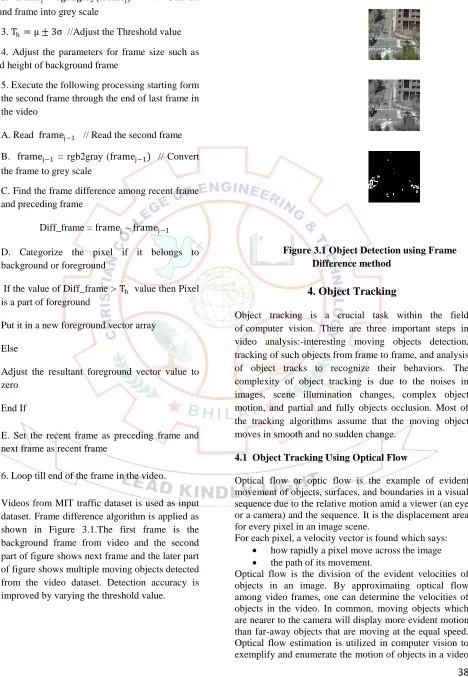
Videos from MIT traffic dataset is used as input dataset. Frame difference algorithm is applied as shown in Figure 3.1.The first frame is the background frame from video and the second part of figure shows next frame and the later part of figure shows multiple moving objects detected from the video dataset. Detection accuracy is improved by varying the threshold value.
Figure 3.1 Object Detection using Frame Difference method
4. Object Tracking
Object tracking is a crucial task within the field of computer vision. There are three important steps in video analysis:-interesting moving objects detection, tracking of such objects from frame to frame, and analysis of object tracks to recognize their behaviors. The complexity of object tracking is due to the noises in images, scene illumination changes, complex object motion, and partial and fully objects occlusion. Most of the tracking algorithms assume that the moving object moves in smooth and no sudden change.
4.1 Object Tracking Using Optical Flow
Optical flow or optic flow is the example of evident movement of objects, surfaces, and boundaries in a visual sequence due to the relative motion amid a viewer (an eye or a camera) and the sequence. It is the displacement area for every pixel in an image scene.
For each pixel, a velocity vector is found which says:
how rapidly a pixel move across the image
the path of its movement.
CCET JOURNAL OF SCIENCE AND ENGINEERING EDUCATION
(ISSN 2455-5061)
Vol. - 3, Page-36-44, Year-2018
39
sequence, frequently for motion-oriented object detection and tracking methods.
The experimentation intensity of every object point is constant over time. These objects points in the image coordinate moves in a same manner (velocity smoothness restriction). Suppose we have a constant image; I {m, n, t) denotes to the gray-level of (m, n) at time t. Characterizing a dynamic image as a function of location and time permits it to be articulated.
Assume every pixel moves however does not change intensity.
Pixel at position (m, n) in frame1 is pixel at (m+Δm, n+Δn) in frame2.
Optic flow correlates displacement vector through every pixel.
The optical flow illustrates the direction and time pixels in a time series of two subsequent
dimensional velocity vector, which carries direction and the velocity of motion, that is allocated to every pixel in a specified position of the picture. For making calculation easier and faster we relocate the real world three dimensional (3-D+time) objects onto a (2-D+time) plane. Then we can explain the image by making use of the 2-D dynamic intensity function of I {m, n, t} making sure that in the neighborhood of pixel, change of intensity does not occur in the motion field, we can use the following expression
I (m, n, t) = I (m +δm, n +δn, t+ δt)……… (4.1)
Using Taylor series for the right hand part of the (1) we obtain
I m +δm, n +δn, t + δt = I m, n, t + 𝜕𝐼 𝜕𝑚δm + 𝜕𝐼
𝜕𝑛δn + 𝜕𝐼
𝜕𝑡δt + H. O. T……… (4. 2)
From (4.11) and (4.12), after neglecting higher order terms (H.O.T.) and with modifications we get
Im. vm+ In. vn =
−It………... (4. 3)
or in formal vector representation
v ==
−It………. (4.4)
where ∇𝐼 is called as the spatial gradient of brightness intensity and v is the optical flow (velocity vector) of the image pixel and Itis the time derivative of the brightness intensity[11].
Thus optical flow can give important information about the spatial arrangement of the objects viewed and the rate of change of this arrangement.
Multiple objects can be tracked easily from the video dataset as shown in Figure 4.1.It shows original video first, then motion vectors calculated can be seen in second window. Third window showing objects segmented due to thresholding and the last window shows multiple objects being tracked.
Figure 4.1 Multiple Object Tracking using Optical Flow from random frame1
5. Object Classification
Classification is process which classifies objects into distinct segments called classes. But unlike clustering, a classification analysis requires that the end-user/analyst know ahead of time how classes are defined.
5.1 Dataset
The system is initialized by inputting video sequence from a static camera monitoring a site. The majority of the techniques are able to work on both color and monochrome video sequence. The first phase is acquiring the images of pedestrians, light vehicles and heavy vehicles. We use pedestrian detection dataset of university of Pennsylvania for person, images from website of Kenworthfor heavy vehicles and images from website of cardekho for light vehicles were used to as input dataset and videos from MIT traffic dataset as test dataset.
CCET JOURNAL OF SCIENCE AND ENGINEERING EDUCATION
(ISSN 2455-5061)
Vol. - 3, Page-36-44, Year-2018
40
basic mathematical morphology operations that are dilation and erosion, based on Minkowski algebra is defined in Equation 5.1 & 5.2[12].
Dilation
D P, Q = P ⊕ Q = βϵQ(P +
β)………..(5.1)
Erosion
E P, Q = P ⊖ (−Q) = βϵQ(P −β)
……….(5.2)
where
−Q = {−Q|βϵQ}
While either set P or Q can be notion of as an "image”, P is generally considered as the image and Q is called a structuring element. In brief dilation makes objects to dilate or grow in size; erosion makes objects to shrink. The quantity and the way that the object grows or shrinks depend upon the choice of the structuring element.
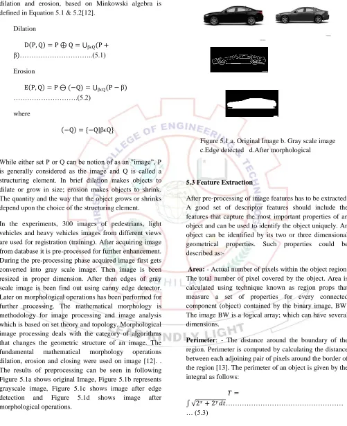
In the experiments, 300 images of pedestrians, light vehicles and heavy vehicles images from different views are used for registration (training). After acquiring image from database it is pre-processed for further enhancement. During the pre-processing phase acquired image first gets converted into gray scale image. Then image is been resized in proper dimension. After then edges of gray scale image is been find out using canny edge detector. Later on morphological operations has been performed for further processing. The mathematical morphology is methodology for image processing and image analysis which is based on set theory and topology. Morphological image processing deals with the category of algorithms that changes the geometric structure of an image. The fundamental mathematical morphology operations dilation, erosion and closing were used on image [12]. . The results of preprocessing can be seen in following Figure 5.1a shows original Image, Figure 5.1b represents grayscale image, Figure 5.1c shows image after edge detection and Figure 5.1d shows image after morphological operations.
Figure 5.1 a. Original Image b. Gray scale image c.Edge detected d.After morphological
5.3 Feature Extraction
After pre-processing of image features has to be extracted. A good set of descriptor features should include the features that capture the most important properties of an object and can be used to identify the object uniquely. An object can be identified by its two or three dimensional geometrical properties. Such properties could be described as:-
Area: - Actual number of pixels within the object region. The total number of pixel covered by the object. Area is calculated using technique known as region props that measure a set of properties for every connected component (object) contained by the binary image, BW. The image BW is a logical array; which can have several dimensions.
Perimeter: - The distance around the boundary of the region. Perimeter is computed by calculating the distance between each adjoining pair of pixels around the border of the region [13]. The perimeter of an object is given by the integral as follows:
𝑇 =
2𝑥+ 2𝑦𝑑𝑡………
… (5.3)
CCET JOURNAL OF SCIENCE AND ENGINEERING EDUCATION
(ISSN 2455-5061)
Vol. - 3, Page-36-44, Year-2018
41
1x,...,nx is a boundary coordinate list, the object perimeter is given by:
𝑇 = 𝑁−1𝑖=1 𝑑𝑖 = 𝑁−1𝑖=1 |𝑥𝑖− 𝑥𝑖+1 |……….. (5.4)
Major Axis: - Major and minor axes are the simplest of all features but yet important. They give essential information of an object such as elongation, eccentricity etc. The major axis points are the two points in an object where the object is more elongated and where the straight line drawn between these two points is the longest. Major axis points are calculated by all possible combinations of perimeter pixels where the line is the longest [13]. The length of the major axis is given by:
𝑀𝑎𝑗𝑜𝑟 𝐴𝑥𝑖𝑠𝑙𝑒𝑛𝑔𝑡ℎ =
(𝑥2− 𝑥1)2+ (𝑦2− 𝑦1)2……… (5.5)
where (x1, y1) and (x2, y2) are the coordinates of the two end points of the major axis.
Minor Axis: - The minor axis is drawn perpendicular to the major axis where this line has the maximum length. Once the end points of the minor axis have been found, its length is given by the same equation as the major axis length. It is also called the object width [13].
𝑀𝑖𝑛𝑜𝑟 𝐴𝑥𝑖𝑠𝑙𝑒𝑛𝑔𝑡ℎ =
(𝑥2− 𝑥1)2+ (𝑦2− 𝑦1)2………...
(5.6)
where (x1, y1) and (x2, y2) are the coordinates of the two end points of the minor axis.
Convex Area: - It specifies the number of pixels in „Convex Image‟ [13]. Whereas Convex Image is binary image (logical) that specifies the convex hull, with all pixels within the hull filled (convex polygon).
Eccentricity: - Eccentricity is the ratio between the lengths of the short axis to the long axis Gonzalez et al. (2004) as defined in the following equation.
𝐸𝑐𝑐𝑒𝑛𝑡𝑟𝑖𝑐𝑖𝑡𝑦 = 𝐴𝑥𝑖𝑠𝑙𝑒𝑛𝑔𝑡 ℎ𝑠ℎ 𝑜𝑟𝑡
𝐴𝑥𝑖𝑠𝑙𝑒𝑛𝑔𝑡 ℎ𝑙𝑜𝑛𝑔 ……… (5.7)
The value of eccentricity is between 0 and 1. Eccentricity is also called ellipticity with respect to minor axis and major axis of the ellipse. If the major axis gets longer, eccentricity gets higher.
Equivdiameter: - specifies the diameter of a circle with the same area as the region[13]. It is computed as:
𝐸𝑞𝑢𝑖𝑣𝑑𝑖𝑎𝑚𝑒𝑡𝑒𝑟 = 4∗𝐴𝑟𝑒𝑎
𝑃𝑖 ……… (5.8)
Solidity: - In simple terms density is mass per unit volume. But in two dimensional image objects this can be defined as the ratio between the area and convex area of the same object [13]:
𝑆𝑜𝑙𝑖𝑑𝑖𝑡𝑦 = 𝐴𝑟𝑒𝑎
𝐶𝑜𝑛𝑣𝑒𝑥𝐴𝑟𝑒𝑎……… (5.9)
CCET JOURNAL OF SCIENCE AND ENGINEERING EDUCATION
(ISSN 2455-5061)
Vol. - 3, Page-36-44, Year-2018
42
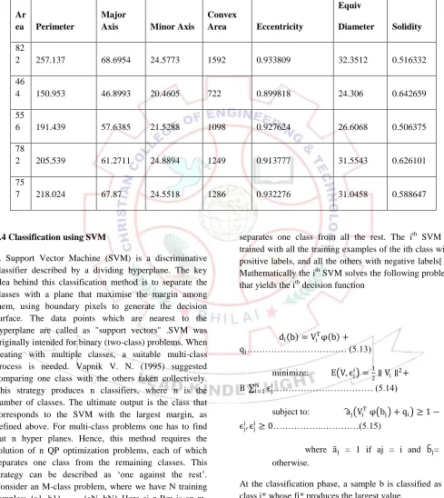
Table 5.1 Sample Dataset
5.4 Classification using SVM
A Support Vector Machine (SVM) is a discriminative classifier described by a dividing hyperplane. The key idea behind this classification method is to separate the classes with a plane that maximise the margin among them, using boundary pixels to generate the decision surface. The data points which are nearest to the hyperplane are called as "support vectors" .SVM was originally intended for binary (two-class) problems. When treating with multiple classes, a suitable multi-class process is needed. Vapnik V. N. (1995) suggested comparing one class with the others taken collectively. This strategy produces n classifiers, where n is the number of classes. The ultimate output is the class that corresponds to the SVM with the largest margin, as defined above. For multi-class problems one has to find out n hyper planes. Hence, this method requires the solution of n QP optimization problems, each of which separates one class from the remaining classes. This strategy can be described as „one against the rest‟. Consider an M-class problem, where we have N training samples: {a1, b1},….., {aN, bN} Here ai ε Rm is an m-dimensional feature vector and bi ε {1, 2,…., M} is the corresponding class label. One-against-all approach constructs M binary SVM classifiers, each of which
separates one class from all the rest. The ith SVM is trained with all the training examples of the ith class with positive labels, and all the others with negative labels[1]. Mathematically the ith SVM solves the following problem that yields the ith decision function
di b = ViTφ b + qi……… (5.13)
minimize: E V, ϵji = 1 2∥ Vi∥
2+ B Nl=1ϵji……… (5.14)
subject to: aj ViT φ bj + qi ≥ 1 − ϵji, ϵji≥ 0………..…………(5.15)
where a j = 1 if aj = i and b j= -1
otherwise.
At the classification phase, a sample b is classified as in class i* whose fi* produces the largest value.
i* = arg max fi(x)=arg max(ViTφ b + qi)……… (5.16)
Ar
ea Perimeter
Major
Axis Minor Axis
Convex
Area Eccentricity
Equiv
Diameter Solidity 82
2 257.137 68.6954 24.5773 1592 0.933809 32.3512 0.516332
46
4 150.953 46.8993 20.4605 722 0.899818 24.306 0.642659
55
6 191.439 57.6385 21.5288 1098 0.927624 26.6068 0.506375
78
2 205.539 61.2711 24.8894 1249 0.913777 31.5543 0.626101
75
CCET JOURNAL OF SCIENCE AND ENGINEERING EDUCATION
(ISSN 2455-5061)
Vol. - 3, Page-36-44, Year-2018
43
where i=1,………….,M.
Thus multiclass SVM classifier was implemented and objects were classified accordingly into multiple classes as pedestrians, light vehicles and heavy vehicles effectively.
6. Performance Evaluation & Result
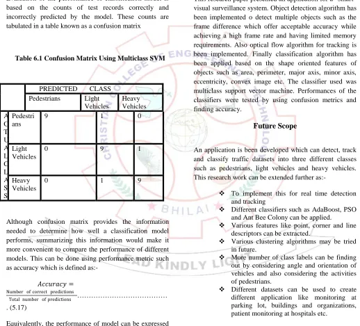
Evaluation of the performance of classification model is based on the counts of test records correctly and incorrectly predicted by the model. These counts are tabulated in a table known as a confusion matrix
Table 6.1 Confusion Matrix Using Multiclass SVM
Although confusion matrix provides the information needed to determine how well a classification model performs, summarizing this information would make it more convenient to compare the performance of different models. This can be done using performance metric such as accuracy which is defined as:-
𝐴𝑐𝑐𝑢𝑟𝑎𝑐𝑦 = Number of correct predictions
Total number of predictions ………
. (5.17)
Equivalently, the performance of model can be expressed in terms of it error rate, which is defined as:-
𝐸𝑟𝑟𝑜𝑟 𝑟𝑎𝑡𝑒 = Number of wrong predictions
Total number of predictions ……….. (5. 18)
Classification algorithms seek models which should attain highest accuracy and eventually lowest error rate when applied to test data set. Multiclass SVM classifier is applied on the dataset which achieves highest accuracy i.e. 90%.
Conclusion
This research paper presented an application for a “smart” visual surveillance system. Object detection algorithm has been implemented o detect multiple objects such as the frame difference which offer acceptable accuracy while achieving a high frame rate and having limited memory requirements. Also optical flow algorithm for tracking is been implemented. Finally classification algorithm has been applied based on the shape oriented features of objects such as area, perimeter, major axis, minor axis, eccentricity, convex image etc. The classifier used was multiclass support vector machine. Performances of the classifiers were tested by using confusion metrics and finding accuracy.
Future Scope
An application is been developed which can detect, track and classify traffic datasets into three different classes such as pedestrians, light vehicles and heavy vehicles. This research work can be extended further as:-
To implement this for real time detection and tracking
Different classifiers such as AdaBoost, PSO and Ant Bee Colony can be applied.
Various features like point, corner and line descriptors can be extracted.
Various clustering algorithms may be tried in future.
More number of class labels can be finding out by considering angle and orientation of vehicles and also considering the activities of pedestrians.
Different datasets can be used to create different application like monitoring at parking lot, buildings and organizations, patient monitoring at hospitals etc.
PREDICTED CLASS Pedestrians Light
Vehicles
Heavy Vehicles A
C T U A L C L A S S
Pedestri ans
9 1 0
Light Vehicles
0 9 1
Heavy Vehicles
CCET JOURNAL OF SCIENCE AND ENGINEERING EDUCATION
(ISSN 2455-5061)
Vol. - 3, Page-36-44, Year-2018
44
References
[1] Lin, D. T., and Chen, Y. T. (2011),‟Pedestrianand Vehicle Classification Surveillance System for Street- Crossing Safety‟, In The 201 International Conference on Image Processing Computer Vision, and Pattern Recognition (IPCV'11).
[2] Jun-Wei ,Hsieh, Shih-Hao Yu, Yung-ShenChen, Wen-Fong Hu.(2006),‟Automatic Traffic Surveillance System for Vehicle Tracking and Classification‟, IEEE transactions on intelligent transportation systems, vol 7, no 2.
[3] Gupte S, Masoud O, Martin R F K Papanikolopoulos, N P. (2002),‟ Detection and Classification of Vehicles‟, IEEE Transactions on Intelligent Transportation Systems, Vol 3, No 1.
[4] Kato T, Ninomiya Y, Masaki I. (2002), ‟Preceding vehicle recognition based on learning from sample images‟, IEEE Transactions on Intelligent Transportation Systems, Vol 3, No 4.
[5] Dubuisson Jolly, MP, Lakshmanan, S, Jain, A K. (1996), ‟Vehicle Segmentation and Classification using Deformable Templates‟, IEEE Transactions on Pattern Analysis and Machine Intelligence, Vol 18, No 3.
[6] Betke, M., Haritaoglu, E., and Davis, L. S. (2000),‟ Real-time multiple vehicle detection and tracking from a moving vehicle‟, Machine Vision and Applications , Vol 12, pp 69-83.
[7] Zhong Qin and Guangzhou. (2008),‟Method of Vehicle Classification Based on Video‟, Proceedings of the IEEE/ ASME International Conference on Advanced Intelligent Mechatronics, Xi‟an, China.
[8] Watve K.Alok,and Dr. Sural Shamik (1998), „Object tracking in video scenes‟, Technical seminar at IIT Kharagpur.
[9] Tiwari Shanik, Kumari Deepa, Gupta Deepika,and Raina(2012), „ Enhanced Military Security Via Robot Vision Implementation Using Moving Object Detection and Classification Methods‟ ,IOSR Journal of Engineering (IOSRJEN), Vol. 2 Issue 1, pp.162-165.
[10] Chaohui, Zhan, Xiaohui Duan, Shuoyu Xu, Zheng Song, and Min Luo (2007), „An Improved Moving Object Detection Algorithm Based on Frame Difference and Edge Detection‟, Fourth International Conference on Image and Graphics, 0-7695-2929-1/07 $25.00 © IEEE, DOI 10.1109/ ICIG. 2007.153
[11] Aslani, S., & Mahdavi-Nasab, H. (2013), „Optical Flow Based Moving Object Detection and Tracking for Traffic Surveillance‟, World Academy of Science,
Engineering and Technology, International Journal of Electrical, Computer, Electronics and Communication Engineering Vol:7 No:9.
[12] Gonzalez R C, Woods R E, Eddins S L.(2004), ‟Digital Image Processing using Matlab‟, Book, Prentice Hall.
[13] Huque Enamul ANM (2006) „Shape Analysis and Measurement for the HeLa cell classification of cultured cells in high throughput screening‟, Thesis submitted to School of Humanities and Informatics University of Skövde, Sweden.