Impacts of Regional Climate Model Spatial
Resolution on Summer Flood Simulation
Mariana Castaneda-Gonzalez
1, Annie Poulin
1, Rabindranarth
Romero-Lopez
2, Richard Arsenault
1, François Brissette
1, Diane Chaumont
3and Dominique Paquin
31 École de technologie supérieure, Montreal, Canada
[email protected], [email protected], [email protected],
2
Universidad Veracruzana, Xalapa, Mexico
3 Consortium Ouranos, Montreal, Canada
[email protected], [email protected]
Abstract
This study aims to evaluate the impact of the Canadian Regional Climate Model’s (CRCM) spatial resolution on summer floods simulation. Four different climate simulations issued from the fourth version of the CRCM (two driven by the Canadian General Circulation Model (CGCM) and two driven by the ERA40c reanalysis) are employed. One simulation at 45 km resolution and another one at 15km resolution for each driver were compared on a daily time-step for the 1960-1990 period. These four simulations are used as inputs for two hydrological models of varying complexity (HSAMI and MOHYSE). Each model is calibrated using three different objective functions based on the Kling-Gupta Efficiency criterion (KGE) to target floods. Two seasonal indices are used to evaluate the CRCM outputs: bias (temperature) and relative bias (precipitation). For the streamflow simulations analysis, the seasonal values of KGE and relative bias are used. The results show an impact of spatial resolution on climate model outputs, on streamflow simulation and flood indicators in the hydrological models. However, other elements such as climate model driver and domain size can influence the results, highlighting the need for further research to assess the impact of spatial resolution on summer floods.
Engineering
Volume 3, 2018, Pages 372–380
1
Introduction
Over the course of the years, catastrophic hydrological events such as droughts and floods have occurred around the world causing intense social and economic impacts. Furthermore, it is anticipated that climate change will modify the hydrological regimes in many world regions. As a result, the number of studies evaluating the potential impact of climate change on extreme hydrological events has increased dramatically. Hydrological modelling and streamflow forecasting thus play an important role in the global and regional economy and in many aspects of social development (Grey & Sadoff, 2007)
The climate change impacts on hydrology are usually evaluated using the climate model outputs as inputs for the hydrological models. During the last decades, numerous global climate models (GCMs) have been developed and downscaled with higher-resolution regional climate models (RCMs) that can improve the representation of climate variables such as precipitation (Teutschbein & Seibert, 2010). Therefore, researchers have thrived to improve climate model resolution as it is thought that the finer scales will allow for a better representation of the hydrological processes for studies at the catchment scale (Hawkins et al., 2013; Lee & Bae, 2016; Teutschbein & Seibert, 2010). The increase in spatial resolution also increases the climate model and hydrological model simulation times, which raises the need to evaluate how increasing resolution in climate modelling impacts the hydrological streamflow simulations. In other words, it is necessary to analyse the effects of the higher climate model resolution on the simulation of hydrological extremes such as floods. Thus, to address this issue, the main objective is to analyse the spatial resolution impact of the fourth version of the Canadian Regional Climate Model (CRCM) on the hydrological modelling of rainfall-driven floods in central and southern Quebec.
2
Data and methodology
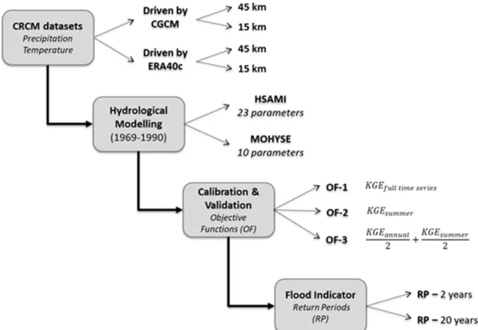
The main parts of the methodology are (1) evaluating the climate outputs (temperature and precipitation), (2) performing the hydrological modelling using the climate datasets from different-resolution CRCM simulations, and (3) computing the summer-fall return periods by a flood frequency analysis using the Gumbel distribution (see Figure 1). This methodology is applied on 50 watersheds in central and southern Quebec over the reference period.
2.1
Climate datasets
Four climate simulations issued from the Canadian Regional Climate Model (CRCM) version 4 (Caya & Laprise, 1999) were used to simulate summer-fall floods (listed in Table1).
Acronym* Pilot Domain Resolution
15km (CGCM) QC CGCM3.1v2 Quebec 15km
45km (CGCM) AMNO CGCM3.1v2 North America 45km
15km (ERA40c) QC ERA40C Quebec 15km
45km (ERA40c) AMNO ERA40C North America 45km
*The acronym stands for: Resolution (Driver) Domain.
Table 1 Description of the climate datasets
2.2
Hydrological modelling
The hydrological simulations were carried out by two different hydrological models of varying complexity. HSAMI (Fortin, 2000) is a lumped, conceptual, rainfall-runoff model with 23 parameters and MOHYSE (Fortin & Turcotte, 2006) is a simplified, lumped, conceptual model with 10 parameters. For the calibration and validation of the hydrological modelling, the KGE (Gupta et al., 2009) (equations (1) – (3)) is the base of the three different objective functions used in this study (see Figure 1). 2 2 2
)
1
(
)
1
(
)
1
(
1
r
KGE
(1)o o s s o s
CV
CV
/
/
(2)o s
(3)Where r is Pearson’s correlation coefficient, α is the variability error, and β represents the bias error. The represents the mean streamflow, CV is the variation coefficient and is the standard deviation of the observed (“o”) and simulated (“s”) streamflows. This KGE criterion measures the
overcome the problems related to the use of functions based on the mean squared error (e.g. runoff peaks and variability underestimation) such as the Nash-Sutcliffe efficiency metric, one of the most commonly used objective functions in hydrological model calibration (Gupta et al., 2009; Nash & Sutcliffe, 1970). Along with it, the KGE increasing popularity in the literature (Beck et al., 2016; Huang et al., 2016; Oyerinde et al., 2017; Thirel et al., 2015), warrants its use in this study.
2.3
Simulations comparison criteria
For the climate outputs analysis, two metrics were used to evaluate the seasonal impact of spatial resolution: bias (temperature) and relative bias (precipitation). For the streamflow, the KGE criterion between streamflow simulations and the relative bias between return periods are used. All comparisons were performed by comparing the differences between the 15 km and 45 km resolutions (presented as 15km/45km), where the 45 km simulation is always used as the reference dataset for climate and streamflow inter comparisons.
3
Results
3.1
Climate simulations
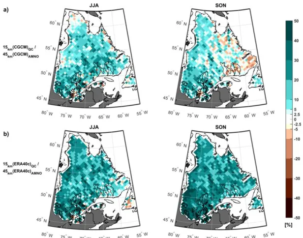
Figures 2 and 3 show the temperature seasonal biases (°C) and the precipitation seasonal relative biases (%) between the simulations at different resolutions, respectively. The figures show the obtained biases for the summer (June, July and August) and fall (September, October and November) seasons over the province of Quebec with the fifty watersheds highlighted in black.
On the comparisons of temperature simulations driven by CGCM (upper panel a in Figure 2) a consistent hot bias is observed during the fall (SON). More variability is observed during the summer (JJA) with a bias varying between +2 and -2 degrees Celsius. On the other hand, the comparisons of the ERA40c-driven simulations (lower panel b) show similar trends in the summer and fall seasons. A general cold bias is observed with some hot spots in the center and southern regions of the province. This is true for both seasons with a slightly hotter bias observed in the center of the province during the summer months.
For precipitation, seasonal relative bias comparisons between the 15 km and 45 km simulations show a consistent wet bias over the entire province for both drivers (see Figure 3). However, on the CGCM-driven simulations (upper panel a) the wet relative biases are smaller than the relative biases on the ERA40c-driven simulations. Also, differences are observed during the fall months of the CGCM-driven simulations. Dryer relative biases are observed on the southeast side of the province, where the largest studied watersheds are located. The ERA40c-driven simulations comparisons (lower panel b) show larger wet biases (up to 50 %) during both seasons.
3.2
Hydrological modelling
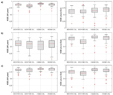
Figure 4 displays the distributions of the Kling-Gupta Efficiency values to evaluate the streamflow simulations against observed streamflows over the full time series (left column) and the during the summer-fall months (right column). The two hydrological models, MOHYSE and HSAMI, present good performance over the fifty watersheds with median KGE values ranging from 0.65 to 0.9 for both calibration and validation periods, and the different objective functions (OF).
Figure 2 Temperature seasonal bias (°C) during the summer (JJA) and fall (SON) seasons for the 1961-1990 period. The upper panels (a) show the comparisons for the datasets driven by CGCM and the lower
panels (b) for the datasets driven by ERA40c
However, during the summer-fall months (right column), both models show difficulties in the streamflow simulations. More outliers and median KGE values close to 0.6 are observed. For OF-2 (b), the hydrological models perform better during June to October. Yet, both hydrological models present a decrease in the median KGE values over the full time series evaluations. For the third calibration approach (c), similar distributions are observed over the full time series and the summer-fall months with slightly better median values in the full time series evaluations (left column).
3.3
Streamflow simulations driven by CRCM4
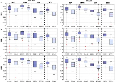
Figure 5 shows the seasonal comparisons of streamflows simulated with climate data at 15 km and 45 km resolutions (using the 45 km as the reference dataset) by using the KGE criterion for the three objective functions (OF) presented on panels a, b and c.
The boxplots show the difference between the streamflows simulated with 15 km and 45 km resolutions for each watershed and both drivers. Larger differences are observed between simulations driven by the ERA40c (light blue) than between simulations driven by the CGCM (dark blue). These differences are observed for all seasons, with the largest differences observed during the summer and
Figure 4 KGE values on the calibration and validation years. Panel a) presents the OF-1, panel b) presents the OF-2 and panel c) presents the OF-3. KGE values for the entire year (left panel) and June to October
(right panel) are shown for both models
fall months (JJA and SON). This tendency is observed for both hydrological models and for the three calibration approaches.
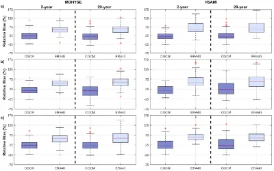
Figure 6 shows the impact of the resolution on the flood frequency indicators. Each boxplot presents the relative biases between the return periods (2-year and 20-year) estimated from the streamflow simulations at 15 km and the 45 km resolution for the different drivers and both hydrological models. The results show an increase on the relative bias with increasing return periods. This is true for both hydrological models and the three objective functions (panels a, b and c).
Overall, the model structure shows small impacts on the results. Small differences are observed between the distributions obtained with both models. Regarding the impacts of hydrological model parameterization, considerable differences are observed in the spread of distributions between the three calibration approaches. The results distributions are noticeably similar for the median values with a few differences in the spread between models. These differences are especially observed in the ERA40c comparisons.
Figure 5 Seasonal KGE values of the comparisons between streamflows generated with climate outputs at 15 km and 45 km resolutions for the four seasons. The upper panels (a) present the results obtained with OF-1,
4
Discussion and conclusion
This research aimed to evaluate the impact of regional climate model spatial resolution on the hydrological modelling of rainfall-driven floods. The results show that the climate model resolution has an impact on temperature and precipitation simulations, which varies from summer to fall seasons. Yet, discrepancies were observed in the temperature biases estimated with the climate simulations issued from the different drivers. On the seasonal precipitation analysis, large relative biases were observed in the precipitation amounts, mainly during the summer season for both drivers. Regarding the hydrological modelling, both hydrological models presented good performance against observations but were shown to be considerably impacted by the use of different objective functions. Nonetheless, HSAMI presented more sensitivity to the different parameter sets. This was expected as the model has more parameters than MOHYSE. Thus, HSAMI’s degrees of freedom allowed the model to adapt the parameters to better simulate the hydrological processes.
On the floods analysis, the flood indicators suggested that impacts on summer-fall floods increased with increasing return periods. Although impacts linked to the climate model resolution were observed, these effects can be due to other elements involved in the climate simulations. The CRCM4 datasets have important differences. They were performed with different drivers (CGCM and ERA40c), and also different domains (Quebec-15km, and North America-45km). Therefore, the attribution of the observed differences in climate datasets, streamflow simulations and flood indicators can be due to the spatial resolution but also to the RCM domains and driver differences. For this reason, it is not possible to link the impacts directly to the spatial resolution. However, these Figure 6 Summer-fall flood return periods (2 and 20 years) relative bias (%) between streamflow simulations
with different resolutions. Panel a) presents the objective function-1, b) the objective function-2 and c) presents the objective function-3
results highlighted the need for further research in order to improve the confidence in our assessment of the impacts of climate model spatial resolution on rainfall-driven floods.
References
Beck, H. E., Dijk, A. I. J. M. v., Roo, A. d., Miralles, D. G., McVicar, T. R., Schellekens, J., & Bruijnzeel, L. A. (2016). Global‐scale regionalization of hydrologic model parameters.
Water resources research, 52(5), 3599-3622. doi:10.1002/2015WR018247
Caya, D., & Laprise, R. (1999). A semi-implicit semi-Lagrangian regional climate model: The Canadian RCM. Monthly Weather Review, 127(3), 341-362.
Fortin, V. (2000). Le modèle météo-apport HSAMI: historique, théorie et application. Institut de recherche d’Hydro-Québec, Varennes.
Fortin, V., & Turcotte, R. (2006). Le modèle hydrologique MOHYSE. Note de cours pour SCA7420, Département des sciences de la terre et de l’atmosphere, Université du Québec a Montréal. Grey, D., & Sadoff, C. W. (2007). Sink or Swim? Water security for growth and development. Water
Policy, 9(6), 545-571.
Gupta, H. V., Kling, H., Yilmaz, K. K., & Martinez, G. F. (2009). Decomposition of the mean squared error and NSE performance criteria: Implications for improving hydrological modelling. Journal of hydrology, 377(1), 80-91.
Hawkins, E., Osborne, T. M., Ho, C. K., & Challinor, A. J. (2013). Calibration and bias correction of climate projections for crop modelling: an idealised case study over Europe. Agricultural and forest meteorology, 170, 19-31.
Huang, S., Kumar, R., Flörke, M., Yang, T., Hundecha, Y., Kraft, P., . . . Krysanova, V. (2016). Evaluation of an ensemble of regional hydrological models in 12 large-scale river basins worldwide. Climatic Change, 141(3), 381-397. doi:10.1007/s10584-016-1841-8
Lee, M.-H., & Bae, D.-H. (2016). Uncertainty Assessment of Future High and Low Flow Projections According to Climate Downscaling and Hydrological Models. Procedia Engineering, 154(Supplement C), 617-623. doi:https://doi.org/10.1016/j.proeng.2016.07.560
Nash, J. E., & Sutcliffe, J. V. (1970). River flow forecasting through conceptual models part I—A discussion of principles. Journal of hydrology, 10(3), 282-290.
Oyerinde, G., Hountondji, F., Lawin, A., Odofin, A., Afouda, A., & Diekkrüger, B. (2017). Improving Hydro-Climatic Projections with Bias-Correction in Sahelian Niger Basin, West Africa.
Climate, 5(1), 8.
Teutschbein, C., & Seibert, J. (2010). Regional climate models for hydrological impact studies at the catchment scale: a review of recent modeling strategies. Geography Compass, 4(7), 834-860. Thirel, G., Andréassian, V., Perrin, C., Audouy, J. N., Berthet, L., Edwards, P., . . . Vaze, J. (2015).