Vol. 10, No. 2, 2018 Article ID IJIM-00835, 9 pages Research Article
An Efficient Schulz-type Method to Compute the Moore-Penrose
Inverse
H. Esmaeili ∗†, R. Erfanifar‡, M. Rashidi §
Received Date: 2016-08-29 Revised Date: 2017-09-27 Accepted Date: 2018-05-17
————————————————————————————————–
Abstract
A new Schulz-type method to compute the Moore-Penrose inverse of a matrix is proposed. Every iteration of the method involves four matrix multiplications. It is proved that this method always converge with fourth-order. A wide set of numerical comparisons shows that the average number of matrix multiplications and the average CPU time of our method are considerably less than those of other methods. For each of sizesn×nandn×(n+ 10),n= 100,200,300,400, ten random matrices were chosen to make these comparisons.
Keywords: Moore-Penrose inverse; Iterative method; Schulz-type method; Fourth-order convergence; Matrix multiplication.
—————————————————————————————————–
1
Introduction
M
adeveloped to compute the Moore-Penroseny higher order iterative methods have been inverse of a matrix. Iterative algorithms are a subject of current research (see, e.g., [11,12, 18,23, 25]), due to the importance of the topic in engineering and applied problems such as linear equations, statistical regression analysis, filtering, signal and image processing, and control of robot manipulators [5,10,15,17].
In this article, we focus on presenting and demonstrating a new method with a close
atten-∗Corresponding author. [email protected], Tel:
+(98)9121028244
†Department of Mathematics, Bu-Ali Sina University,
Hamedan, Iran.
‡Department of Mathematics, Malayer University,
Malayer, Iran.
§Department of Mathematics, Bu-Ali Sina University,
Hamedan, Iran.
tion to reducing the computational time. To this end, we investigate a convergent iterative method to find the Moore-Penrose inverse, which could be viewed as an extension of the famous Schulz method for such a purpose. It is proved that this method always converge with fourth-order, and every iteration involves four matrix multiplica-tions. A theoretical discussion will also be given to show the behavior of the proposed scheme.
In the simple case, when A is a n×n nonsin-gular matrix, to compute the matrix inverse, var-ious iterative methods, called Schulz-type meth-ods, were developed [1,4,6,9,11,13,16,19,22,
24,25], almost all of which are based on iterative solvers for the scalar equation f(x) = 1x −a= 0 applied to the matrix equation
f(X) =X−1−A= 0.
We should also point out that even if the ma-trixA is singular, these methods converge to the
Moore-Penrose inverse using a proper initial ma-trix. A full discussion on this feature of this type of iterative methods has been given in [1,2].
The rest of this paper is organized as follows. Section 2 is devoted to presenting some exist-ing iterative schemes to find the Moore-Penrose inverse. We propose our new method in Sec-tion 3 and prove that it is fourth-order conver-gent. In Section 4, some numerical examples are given to show the performance of the presented method compared with other higher order meth-ods. For each of sizes n×n and n×(n+ 10),
n= 100,200,300,400, ten random matrices were chosen to make these comparisons. Finally, some conclusions are outlined in Section 5.
2
Schulz-type iterative methods
The MoorePenrose inverse of a matrixA∈Cm×n, denoted by A† ∈ Cn×m, is a unique matrix X
satisfying the following four Penrose equations
AXA=A, (AX)∗=AX, XAX=X, (XA)∗=XA,
whereA∗ is the conjugate transpose of A. There are various iterative methods, called Schulz-type methods, to computeA†. In the sequel, we recall some of them.
Perhaps, the most frequently used iterative method to approximate A† is the famous New-ton method
Bk=AXk
Xk+1=Xk(2I−Bk),
(2.1)
originated in [16], in whichI is them×midentity matrix. Schulz in [16] found that the eigenvalues of I −AX0 must have magnitudes less than 1
to ensure the convergence. Since the residuals
Rk =I−AXkin each step (2.1) satisfy∥Rk+1∥≤
∥A∥ ∥Rk∥2, the Newton method is a second-order iterative method [1]. Similarly, in [11] the relation
∥AEk+1∥≤ ∥AEk∥2 is verified for errors of the
form Ek=Xk−A†.
Li et al. in [8] investigated the following third-order method, known as Chebyshev method,
Bk=AXk
Xk+1=Xk(3I−Bk(3I −Bk)),
(2.2)
and also proposed another iterative method to find A† of the same order as given in
Bk=AXk
Xk+1=Xk[I+ 0.5(I−Bk)
(I+ (2I−Bk)2)].
(2.3)
Toutounian and Soleymani [24] proposed the fol-lowing fourth-order method:
Bk=AXk
Xk+1= 0.5Xk[9I −Bk(16I− Bk(14I −Bk(6I−Bk))))].
(2.4)
Krishnamurthy and Sen [7] provided the following fourth-order method:
Xk+1 =Xk(I +Yk(I+Yk(I+Yk))), (2.5)
in which Yk = I−AXk. As another example, a
ninth-order method could be presented as
Xk+1=Xk[I+Yk(I+Yk(I+Yk(I+ Yk(I+Yk(I+Yk(I+Yk(I+Yk)))))))].
The number of matrix-matrix multiplications of the above method can be reduced from 9 to 7 if rewritten as follows:
Bk=Yk2, Ck =Bk2, Dk=Ck2,
Xk+1=Xk[(I+Yk)(I+Bk)(I+Ck) +Dk].
(2.6) Soleymani et al. [21] provided the following sixth-order method:
Bk=AXk
Sk=Bk(−I+Bk)
Xk+1=Xk(2I−Bk)(3I−2Bk+Sk)(I+Sk).
(2.7) Soleymani and Stanimirovi´c [19] investigated the following ninth-order method:
Bk=AXk
Sk=−7I+Bk(9I +Bk(−5I+Bk)) Tk=BkSk
Xk+1=−0.125XkSk(12I+Tk(6I +Tk)).
(2.8) Also, Soleymani et al. [22] proposed another ninth-order method as
Bk=AXk
Sk= 3I +Bk(−3I+Bk)
Tk=BkSk
Xk+1=−19XkSk[−29I+Tk(33I+ Tk(−15I+ 2Tk))].
Recently, Esmaeili and Pirnia [6] investigate a quadratically convergent method as follows:
Bk=AXk
Xk+1=Xk(5.5I−Bk(8I−3.5Bk)).
(2.10)
Although their method is not a higher method, numerical experiments showed that (2.10) is very effective than other methods both in number of matrix multiplications and CPU time.
To start each of methods, we need an initial matrix X0. A discussion on choosing the initial
approximationX0 is given in [2,14]. Perhaps, in
general, the simplest choice for X0 is
X0=βA∗, (2.11)
in which β is a suitable real number.
3
The New Method
In this paper, we would like to propose a fourth-order class of Schulz-type methods to findA†such that is more effective than all of above methods in terms of number of matrix multiplications and CPU time. To this end, we consider the following iterative class of methods:
Bk=AXk Xk+1=Xk
(
aI+bBk+cBk2+dBk3+eBk4
)
,
(3.12) in which a, b, c, d, e are parameters. Note that every iteration of the method (3.12) involves four matrix multiplications. In the sequel, we prove that the method (3.12) is fourth-order convergent toA† for appropriate chooses of parameters.
Note that, using mathematical induction, it would be easy to check that the iterates produced at each cycle of (3.12) satisfy the following rela-tions:
(AXk)∗=AXk, A†AXk=Xk,
(XkA)∗=XkA, XkAA†=Xk.
(3.13)
We can study the convergence properties of the algorithm (3.12) using the error matrix Ek =
Xk−A†. The matrix formula representing Ek+1
is a sum of possible zero-order term consisting of a matrix which does not depend upon Ek, one or more first-order matrix terms in which Ek or Ek∗ appears only once, one or more second-order
terms in which Ek and Ek∗ appear at least twice,
and so on [15]. To compute error estimates, first note that
A†AEk=Ek, EkAA†=Ek,
according to (3.13). Therefore,
XkBk=A†+ 2Ek+EkAEk,
XkBk2=A†+ 3Ek+ 3EkAEk+ (EkA)2Ek, XkBk3=A†+ 4Ek+ 6EkAEk+ 4(EkA)2Ek
+(EkA)3Ek,
XkBk4=A†+ 5Ek+ 10EkAEk+ 10(EkA)2Ek
+5(EkA)3Ek+ (EkA)4Ek.
Now, substituting Xk = A†+Ek in (3.12), we
have
A†+Ek+1= (a+b+c+d+e)A†
+(a+ 2b+ 3c+ 4d+ 5e)Ek
+(b+ 3c+ 6d+ 10e)EkAEk
+(c+ 4d+ 10e)(EkA)2Ek
+(d+ 5e)(EkA)3Ek
+e(EkA)4Ek.
Fourth-order convergent is obtained when
a+b+c+d+e= 1
a+ 2b+ 3c+ 4d+ 5e= 0
b+ 3c+ 6d+ 10e= 0
c+ 4d+ 10e= 0,
that result in
a= 4 +e, b=−(6 + 4e), c= 4 + 6e, d=−(1 + 4e) .
So, we have
Ek+1= (e−1)(EkA)3Ek+e(EkA)4Ek. (3.14)
Hence, the following theorem can be obtained.
Theorem 3.1 Let A be a m×n nonzero com-plex matrix. Moreover, suppose that the initial approximationX0 is defined by (2.11). If the real number β is chose such that
then the iterative method (3.12) converges to A† with fourth-order. Its first, second, third, fourth and fifth order error terms are given by
error1 =error2 =error3 = 0, error4 = (e−1)(EkA)3Ek, error5 =e(EkA)4Ek.
(3.15)
in whichEk =Xk−A†denotes the error matrix. Proof. We can immediately derive (3.15) from (3.14). Furthermore, (3.14) results in
AEk+1 = (e−1)(AEk)4+e(AEk)5.
Hence,
∥AEk+1∥≤(e−1 +e∥AEk∥)∥AEk∥4,
and therefore ∥AEk∥→ 0, since ∥AE0∥< 1. On
the other hand,
∥Ek+1∥=∥A†AEk+1∥≤ ∥A†∥ ∥AEk+1∥
≤ ∥A†∥(e−1 +e∥AEk∥)∥AEk∥4
results in
∥Ek+1∥≤ [
∥A†∥ ∥A∥4(e−1 +e∥A∥ ∥Ek∥)]∥Ek∥4.
Consequently, Xk →A† and the order of
conver-gence is four. 2Now, suppose thatrank(A) =
r ≤ min{m, n} and consider the singular value decomposition ofA as follows:
A=U
[
S 0 0 0
]
V∗, S=diag(σ1, . . . , σr),
σ1 ≥ · · · ≥σr>0.
It is well known that
A†=V
[
S−1 0 0 0
]
U∗.
If we take X0 as (2.11), then
X0 =βA∗ =V [
S0 0
0 0
]
U∗,
where
S0 =βS
is a diagonal matrix. Therefore,
V∗X0U = [
S0 0
0 0
]
.
Now, the principle of mathematical induction and (3.13) lead to
V∗XkU =
[
Sk 0 0 0
]
, (3.16)
in which Sk = diag(s(1k), . . . , s(rk)) is a diagonal
matrix satisfying the following relation:
Sk+1=Sk[(4 +e)I−(6 + 4e)SSk
+(4 + 6e)(SSk)2−(1 + 4e)(SSk)3
+e(SSk)4].
(3.17) Therefore, the diagonal matrices Dk := SSk = diag(d(1k), . . . , d(rk)), where d(ik) =σis(ik), satisfy
Dk+1:=g(Dk) = (4 +e)Dk−(6 + 4e)Dk2
+(4 + 6e)Dk3−(1 + 4e)Dk4+eDk5,
that means
di(k+1)=g(di(k)) = (4 +e)d(ik)
−(6 + 4e)di(k)2+ (4 + 6e)d(ik)3
−(1 + 4e)d(ik)4+ed(ik)5.
(3.18)
In the following theorem, we show that, fore= 8, the sequences (3.18) are fourth-order convergent todi= 1 for any d(0)i ∈(0,1.45).
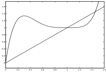
Theorem 3.2 For any initial point d(0) ∈
(0,1.45), the sequence d(k+1) =g(d(k)) is fourth-order convergent to d= 1, in which the function g(x) is defined by
g(x) = 12x−38x2+ 52x3−33x4+ 8x5. (3.19)
Proof. We can find the real fixed points and the critical points of g(x) as follows:
g(x) =x =⇒ x= 0, 1, 1.45, g′(x) = 0 =⇒ x= 0.3, 1, 1, 1.
Noting g′′(0.3) < 0 and g(4)(1) > 0, we can deduce that 0.3 is a local maximizer and 1 is a local minimizer of g(x). On the other hand,
g(0) = 0< 1 =g(1) and g(0.3)≈1.34 <1.45 =
g(1.45). Therefore, x = 0,1 and x = 0.3,1.45 are minimizers and maximizers of g(x) in the in-terval [0,1.45], respectively. Moreover, the in-terval [0,1.45] maps into itself by the function
g(x). Considering an arbitrary initial pointd(0) ∈
Table 1: Convergence order and number of matrix multiplications for different methods
Method (2.1) (2.2) (2.3) (2.4) (2.5) (2.6) (2.7) (2.8) (2.9) (2.10) (3.20)
Convergence
order 2 3 3 4 4 9 6 9 9 2 4
Matrix
multiplications 2 3 4 5 4 7 5 7 7 3 4
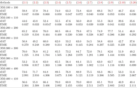
Table 2: Average values of matrix multiplications and elapsed times for different methods
Methods (2.1) (2.2) (2.3) (2.4) (2.5) (2.6) (2.7) (2.8) (2.9) (2.10) (3.20)
DIM:100×100
MAT 59.8 57.9 70.4 74.0 63.2 72.8 63.0 69.3 70.7 46.7 43.6
TIME 0.047 0.038 0.060 0.050 0.047 0.072 0.040 0.050 0.053 0.034 0.036
DIM:100×110
MAT 44.6 43.8 52.4 55.5 47.6 56.0 48.0 55.3 56.0 39.6 35.6
TIME 0.037 0.033 0.0547 0.036 0.038 0.053 0.039 0.039 0.041 0.032 0.031
DIM:200×200
MAT 65.2 63.6 76.0 80.5 68.4 79.8 67.5 74.9 77.7 51.4 46.8
TIME 0.319 0.316 0.464 0.400 0.330 0.560 0.338 0.367 0.386 0.260 0.292
DIM:200×210
MAT 50.8 49.2 60.0 62.0 53.2 63.0 54.5 58.8 63.0 42.7 37.6
TIME 0.270 0.248 0.380 0.314 0.264 0.445 0.284 0.297 0.325 0.239 0.234
DIM:300×300
MAT 70.0 76.8 81.2 85.5 73.2 84.7 72.0 79.1 82.6 51.9 49.2
TIME 1.225 1.184 1.764 1.505 1.263 2.078 1.281 1.380 1.444 0.916 1.086
DIM:300×310
MAT 53.2 51.6 62.0 65.5 56.4 64.4 55.5 63.0 63.7 44.5 40.0
TIME 0.956 0.917 1.363 1.166 0.988 1.589 1.002 1.114 1.116 0.983 0.899
DIM:400×400
MAT 73.6 71.7 84.8 89.5 76.8 88.9 75.5 83.3 86.1 53.3 51.6
TIME 2.991 2.916 4.306 3.675 3.100 5.121 3.119 3.386 3.505 2.189 2.667
DIM:400×410
MAT 56.6 55.8 66.4 70.0 60.0 70.0 60.0 65.1 70.0 46.9 40.4
TIME 2.364 2.308 3.406 2.892 2.455 4.034 2.511 2.675 2.883 2.012 2.111
• The unique solution of the equationg(x) = 1 in the interval [0,1) is 18.
• The functiong(x) is increasing in the interval (0,18). Therefore, if d(k) ∈ (0,18), for some
k, then there exists an index k0 ≥ k such
that eitherd(k0) = 1
8, and so d
(k0+1) = 1, or
d(k0+1) ∈(1
8,1).
• If d(k) ∈ (81,1), for some k, then d(k+1) ∈
(1,1.45).
• If d(k) ∈ (1,1.45), for some k, then the se-quence {d(k+ℓ)}ℓ≥1 ⊆ [1,1.45) is a strictly
decreasing sequence converging tod= 1. Noting the above assertions, we can conclude that
the sequenced(k+1)=g(d(k)) is convergent tod=
1. On the other hand, g′(1) =g′′(1) =g′′′(1) = 0 implies that the convergence is fourth-order (See [3]). 2
Using the iteration function (3.19), we obtain the following iterative method to findA†:
Xk+1=Xk[12I−38(AXk) + 52(AXk)2
−33(AXk)3+ 8(AXk)4],
which can be written as follows:
Bk=AXk Ck=Bk2
Xk+1=Xk[12I−38Bk
+Ck(52I−33Bk+ 8Ck)].
0 0.2 0.4 0.6 0.8 1 1.2 1.4 1.6 0
0.2 0.4 0.6 0.8 1 1.2 1.4 1.6
Figure 1: Graphs of the liney=xand the func-tiony=g(x).
Considering Theorem 3.2, we conclude that if βσ21 = d(0)1 ∈ (0,1.45), then βσi2 = d(0)i ∈
(0,1.45), for alli, and
lim
k→∞Dk =I.
Hence,
lim
k→∞Sk=S −1,
so
lim
k→∞Xk =A †.
Moreover, the order of convergence is four. Therefore, the following theorem is proved.
Theorem 3.3 Consider the m×n complex ma-trixA of rank r, and suppose thatσ21 denotes the largest singular value of A. Moreover, assume that the initial approximation X0 is defined by (2.11), in which
0< β < 1.45
σ21 . (3.21)
Then, the sequence{Xk}k≥0 generated by (3.20)
converges toA†with fourth-order.
Remark 3.1 Consider the initial matrix X0
given in (2.11), with β from (3.21). Since σ12
is a (the) largest singular value of A, we have
σ12 = ∥A∥22≤ ∥A∥1∥A∥∞. Therefore, the
selec-tion
β = 1
∥A∥1∥A∥∞
(3.22)
satisfies (3.21). Furthermore, it is proved in [4] that for such aβ, we have ∥A(X0−A†)∥<1.
Note that every iteration of the method (3.20) involves four matrix multiplications. Although
(3.20) is not a higher order scheme, the numer-ical experiments show that its total number of matrix multiplications and its CPU time are con-siderably less than those of other methods. So, method (3.20) will be the fastest one among con-sidered iterative methods in this article.
The Schulz-type iterations, including (3.20), are strongly numerically stable, that is, they have the self-correcting characteristic and are essen-tially based upon matrix multiplication per an iterative step. The iterative scheme (3.20) could be combined efficiently with sparse techniques in order to reduce the computational load of matrix multiplications per step.
Remark 3.2 If m ≤ n, then we apply (3.20) in the same form, in whichI denotes the m×m
identity matrix. On the other hand, for m > n
we must apply (3.20) with A∗ instead of A and use the n×n identity matrix. So, for the case
m > n, we compute (A∗)†, that is (A†)∗.
Theorem 3.4 If the same assumptions as in Theorem 3.3 are considered, then the use of the iterative method (3.20) for finding the Moore-Penrose generalized inverse has an asymptotical stability.
Proof. The steps of proving the asymptotic sta-bility of (3.20) are similar to those taken for a gen-eral family of methods in [20]. Hence, the proof is omitted. 2
4
Numerical experiments
In this section, we will make some numerical comparisons of our proposed method (3.20) with other methods presented here. To this end, we fo-cus on the total number of matrix multiplications and CPU times required for convergence. Table 1 denotes the number of matrix multiplications in any iteration of different methods.
All tests were carried out with Matlab, while the computer specifications are Microsoft Win-dows XP Intel(R), Pentium(R) 4, CPU 2.60 GHz, with 2 GB of RAM.
We used the initial matrixX0 defined in (2.11),
withβ from (3.21). The stop criterion was
∥Xk+1−Xk∥∞
1 +∥Xk∥∞
and the maximum number of iterations was set to 100. Following [6,21, 24], for each of sizes n×n
and n×(n+ 10),n= 100,200,300,400, we have performed 10 random tests and compared aver-age values of matrix multiplications and elapsed times in seconds. The results are listed in Table
2, where DIM, MAT, and TIME denote the size ofA, average values of matrix multiplications and elapsed times in seconds, respectively.
From Table 2, we observe that the method (3.20) is much better than others both in matrix multiplications and CPU time. The worst one is the ninth-order method (2.4). The third-order method (2.2) and the second-order method (2.1) are better than the higher order methods, al-though they are not comparable with our method. We can almost arrange these methods in the form
{(2.4),(2.6)}<{(2.3),(2.8),(2.9)}<
{(2.5),(2.7)}<{(2.1)}<{(2.2)} ≪
{(2.10)}<{(3.20)},
meaning that methods belonging to a set have a similar efficiency, while ”<” denotes less effi-ciency.
5
Conclusions
In this paper, we proposed a new Schulz-type method to find the Moore-Penrose inverse. It was proved that the method converge with fourth-order. Although our method is not a higher order scheme, a wide set of random numerical experi-ments showed that the required number of ma-trix multiplications and CPU time is considerably less than those of higher order methods. So, our method could be considered as a fast method.
References
[1] A. Ben-Israel, D. Cohen, On iterative com-putation of generalized inverses and associ-ated projections, SlAM J. Numer. Anal. 3 (1966) 410-419.
[2] A. Ben-Israel, T. N. E. Greville, Gen-eralized Inverses, 2nd ed., CMS Books Math./OuvragesMath.SMC 15, Springer,
New York, (2003).
[3] R. L. Burden, J. D. Faires, Numerical Anal-ysis, 9th ed., Brooks/Cole,Boston, (2011). [4] H. Chen, Y. Wang, A family of higher-order
convergent iterative methods for comput-ing the MoorePenrose inverse, Appl. Math. Comput.218 (2011) 4012-4016.
[5] A. Cichocki, B. Unbehauen, Neural networks for optimization and signal processing, New York, John Wiley & Sons, (1993).
[6] H. Esmaeili, A. Pirnia, An efficient quadrati-cally convergent iterative method to find the Moore-Penrose inverse,Int. J. Comp. Math.
94 (2017) 1079-1088.
[7] E. V. Krishnamurthy, S. K. Sen, Numerical Algorithms. Computations in Science and Engineering, Affiliated East-West Press Pvt.
New Delhi, (1986).
[8] H. B. Li, T. Z. Huang, Y. Zhang, X.P. Liu, T.X. Gu, Chebyshev-type methods and pre-conditioning techniques, Appl. Math. Com-put.218 (2001) 260-270.
[9] W. Li, Z. Li, A family of iterative methods for computing the approximate inverse of a square matrix and inner inverse of a non-square matrix, Appl. Math. Comput. 215 (2010) 3433-3442.
[10] S. Miljkovi´c, M. Miladinovi´c, P., Stan-imirovi´c, I. Stojanovi´c, Application of the pseudo-inverse computation in reconstruc-tion of blurred images, Filomat 26 (2012) 453-465.
[11] H. S. Najafi, M. S. Solary, Computational algorithms for computing the inverse of a square matrix, quasi-inverse of a non-square matrix and block matrices, Appl. Math. Comput.183 (2006) 539-550.
[12] V. Y. Pan, R. Schreiber, An improved New-ton iteration for the generalized inverse of a matrix with applications,SIAM J. Sci. Stat. Comput.12 (1991) 1109-1131.
[14] V. Y. Pan, Structured Matrices and Polynomials, Unified Superfast Algorithms, Birkhauser-Springer,New York, (2001).
[15] P. Roland, P. B. Graben, Inverse problems in neural field theory, SIAM J. Appl. Dynam. Sys.8 (2009) 1405-1433.
[16] G. Schulz, Iterative Berechmmg der rezipro-ken Matrix, Z. Angew. Math. Mech. 13 (1933) 57-59.
[17] L. Sciavicco, B. Siciliano, Modelling and control of robot manipulators, London, Springer–Verlag, (2000).
[18] X. Sheng, G. Chen, The generalized weighted MoorePenrose inverse, J. Appl. Math. Comput.25 (2007) 407-413.
[19] F. Soleymani, P. S. Stanimirovi´c, A Higher Order Iterative Method for Computing the Drazin Inverse, The Scientific World Jour-nal Volume 2013, Article ID 708647, 11 pages http://dx.doi.org/10.1155/2013/ 708647/.
[20] F. Soleymani, P. S. Stanimirovi´c, A note on the stability of ap-th order iteration for find-ing generalized inverses,Appl. Math. Lett.28 (2014) 77-81.
[21] F. Soleymani, P. S. Stanimirovi´c, M.Z. Ul-lah, An accelerated iterative method for computing weighted MoorePenrose inverse,
Appl. Math. Comput.222 (2013) 365-371.
[22] F. Soleymani, H. Salmani, M. Rasouli, Find-ing the MoorePenrose inverse by a new matrix iteration, Appl. Math. Comput. 47 (2015) 33-48.
[23] S. Srivastava, D.K. Gupta, A higher order it-erative method forA(2)T,S,Appl. Math. Com-put., (2013) http://dx.doi.org/10.1007/ s12190-013-0743-4/.
[24] F. Toutounian, F. Soleymani, An iterative method for computing the approximate in-verse of a square matrix and the MoorePen-rose inverse of a non-square matrix, Appl. Math. Comput.224 (2013) 671-680.
[25] L. Weiguo, L. Juan, Q. Tiantian, A family of iterative methods for computingMoorePen-rose inverse of a matrix,Linear Algebr. Appl.
438 (2013) 47-56.
Hamid Esmaeili is Associate Pro-fessor of applied mathematics and Faculty of Sciences, Bu-Ali Sina University, Hamedan, Iran. His re-search interests include Optimiza-toin, Numerical Analysis, and Nu-merical Linear Algebra. He has published more than 30 papers in international journals and conferences.
Raziyeh Erfanifar is now PhD student of applied mathematics, Malayer University, Malayer, Iran. Her research interests include frac-tional calculus, numerical analysis, and numerical linear algebra. He has published some papers in in-ternational journals and conferences.