Vol. 10, No. 1, 2018 Article ID IJIM-01050, 8 pages Research Article
A Numerical Method For Solving Physiology Problems By Shifted
Chebyshev Operational Matrix
E. Hashemizadeh ∗†, F. Mahmoudi ‡
Received Date: 2017-03-22 Revised Date: 2017-08-18 Accepted Date: 2017-10-22
————————————————————————————————–
Abstract
In this study, a new numerical solution of singular nonlinear differential equations, stemming from biology and physiology problems, is proposed. The methodology is primarily based on the shifted Chebyshev polynomials operational matrix of derivative and collocation. Furthermore, the conver-gence analysis on the proposed method is carried out. To assess the accuracy and analysis of perfor-mance of the method, five numerical problems, based on the singular nonlinear differential equations, on different subjects, such as the human head, Oxygen diffusion in a spherical cell and Bessel dif-ferential equation, were solved. The numerical results were compared with other existed methods in tables for verification and further discussions.
Keywords: Differential equations; Shifted Chebyshev polynomials; Operational matrix of derivative; Convergence analysis; Physiology problems.
—————————————————————————————————–
1
Introduction
T
hplications in fluid mechanics, biology, physicse differential equations arise from various ap-and engineering [1]-[16]. Such equations also ap-pear in electromagnetic and electrodynamic, elas-ticity and dynamic contact, heat and mass trans-fer, fluid mechanic, acoustic, chemical and elec-trochemical processes, molecular physics, popu-lation, medicine and in many other fields [3]-[14]. For numerical solution of the differential equa-tions, there are some well-known numerical meth-ods [11]-[15].In this paper, we consider the singular
prob-∗Corresponding author. [email protected] , Tel: +98(26)34182389.
†Young Researchers and Elite Club, Karaj Branch, Is-lamic Azad University, Karaj, Iran.
‡Young Researchers and Elite Club, Karaj Branch, Is-lamic Azad University, Karaj, Iran.
lems of the type
y′′(x) +p(x)y′(x) +q(x)y(x) =g(x), 0< x≤1,
(1.1) subject to the conditions
{
α1y(0) +β1y′(0) =γ1,
α2y(1) +β2y′(1) =γ2,
(1.2)
where x = 0 is a singular point in p(x), also
p(x), q(x) and g(x) are continuous functions on (0,1] and the parameters α1, α2, β1, β2, γ1, γ2 are real constants.
The Chebyshev polynomials have been in exis-tence for over a hundred years and they have been used for solving many different problems [2].
In this paper, we propose a suitable way to approximate the solution of singular nonlinear differential equations with initial or boundary value problems on the interval (0, L), by use of shifted Chebyshev collocation method based on the shifted Chebyshev operational matrix ot
derivative. Also the convergence analysis of the proposed method is discussed in this paper.
This paper is organized as follows: In section 2, the shifted Chebyshev polynomials with their properties are introduced. In section 3, we de-rive an approximate formula for derivatives us-ing shifted Chebyshev polynomials and estimate proposed formula. In section 4, we give the er-ror analysis for the method. In section 5, the proposed method is applied to several examples. Finally Section6 concludes the paper with some remarks.
2
Properties of Shifted
Cheby-shev Polynomials
The well known Chebyshev polynomials are de-fined on the interval [−1,1] and can be deter-mined with the aid of the following recurrence formula [2,4]:
Tn+1(x) = 2xTn(x)−Tn−1(x), n= 1,2,· · · (2.3) where T0(x) = 1 and T1(x) = x. The analytic form of the Chebyshev polynomial of degreen is given by :
Tn(x) = n 2 [n 2] ∑ r=0
(−1)r(n−r−1)!
r! (n−2r)!(2x)
n−2r. (2.4)
In order to apply the Chebyshev polynomials in the interval [0,1], we defined the so called shifted Chebyshev polynomials by introducing the change of variablet= 2Lx−1. Let the shifted Chebyshev polynomialsTi(2Lx−1) be denoted by TL,i(x). ThenTL,i(x) can be generated by using the following recurrence relation:
TL,i+1(x) = 2( 2x
L −1)TL,i(x)−TL,i−1(x), i= 1,2,· · ·
(2.5)
whereTL,0(x) = 1 andTL,1(x) = 2Lx−1. The an-alytic from of the shifted Chebyshev polynomials
TL,i(x) of degreeiis given by
TL,i(x) =i i ∑
k=0
(−1)i−k(i+k−1)! 2 2k
(i−k)! (2k)!Lkx
k, (2.6)
where TL,i(0) = (−1)i and TL,i(L) = 1. The or-thogonality condition is
∫ L
0
TL,k(x)TL,j(x)WL(x)dx=hkδjk, (2.7)
where WL(x) = √Lx1−x2 and hk = ϵk
2π, with
ϵ0 = 2, ϵi = 1, i ≥1. Any function u(x), square integrable in (0, L), may be expressed in terms of shifted Chebyshev polynomials as
u(x) = Σ∞j=0ajTL,j(x), (2.8)
where the coefficients aj are given by
aj = 1
hj ∫ L
0
u(x)TL,j(x)WL(x)dx, j = 0,1,2,· · ·
(2.9) In practice, only the first (N + 1)-terms shifted Chebyshev polynomials are considered. Hence, if we write
u(x)≃ΣNj=0cjTL,j(x) =CTϕ(x), (2.10)
where shifted Chebyshev polynomials coefficient vectorC and the shifted Chebyshev polynomials vectorϕ(x) are given by
CT = [c0, c1, . . . , cN], (2.11)
ϕ(x) = [TL,0(x), TL,1(x), . . . , TL,N(x)]T, (2.12)
then the derivative of the vector ϕ(x) can be ex-pressed by [4]
dϕ(x)
dx =D
1ϕ(x), (2.13)
where D1 is the (N + 1)×(N + 1) operational matrix of derivative given by
D1 = (dij) = {
4i
ϵjL, i=j+k,
0, otherwise. (2.14)
IfN is odd k= 1,3,5,· · ·, N, ifN is even k= 1,3,5,· · ·, N−1, for example for evenN, we have
D1 as follows:
2 L
0 0 0 0 · · · 0 0
1 0 0 0 · · · 0 0
0 4 0 0 · · · 0 0
3 0 6 0 · · · 0 0
0 8 0 8 · · · 0 0
5 0 10 0 · · · 0 0
..
. ... ... ... ... ... ...
N−1 0 2N−2 0 · · · 0 0
0 2N 0 2N · · · 2N 0
By using Eq. (2.3), it is clear that
dnϕ(x) dxn = (D
1)nϕ(x), (2.16)
wheren∈N and the superscript, inD(1), denotes matrix power thus
D(n)= (D(1))n, n= 1,2,· · · (2.17)
3
Implementation
of
Shifted
Chebyshev
Polynomials
Method on Physiology
Prob-lems
In this section we use shifted Chebyshev vector and its operational matrix of derivative to solve nonlinear singular boundary value problem of the form Eqs. (2)-(3), we approximatey(x) andg(x) by Chebyshev polynomials as
y(x)≃CTϕ(x), (3.18)
g(x)≃GTϕ(x), (3.19)
we have
y′(x)≃CTD1ϕ(x), (3.20)
y′′(x)≃CT(D1)2ϕ(x), (3.21)
by employing Eqs. (3.18)-(2.13) in Eq. (2) we have
CT(D′)2ϕ(x) +p(x)CTD′ϕ(x)+
q(x)(CTϕ(x)) =GTϕ(x). (3.22)
Also by using Eqs,(3),(3.18) and (3.20) we have
α1CTϕ(0) +β1CTD1ϕ(0) =γ1, (3.23)
α2CTϕ(1) +β2CTD1ϕ(1) =γ2. (3.24)
Equations (3.23) and (3.24) give 2 linear equa-tions. Since the total unknowns for vector C in Eq. (3.22) areN + 1, we collocate that in N−1 roots of Chebyshev polynomials as:
xp= cos pπ
2N, p= 1, . . . , N−1. (3.25)
Then we have Eq. (3.22) as following system of nonlinear equations
CT(D′)2ϕ(xp) +p(xp)CTD′ϕ(xp)+
q(xp)(CTϕ(xp)) =GTϕ(xp),
p= 1,2· · ·, N −1.
(3.26)
Now the resulting Eqs. (3.23), (3.24) and (3.26) generate a system ofN+ 1 nonlinear equa-tions which can be solved using Newton’s itera-tive method. So we have the approximate solu-tion of Eq. (2) with the initial conditions (3) by Chebyshev polynomials as:
ym(x) = N ∑
j=0
cjTL,j(x) =CTϕ(x). (3.27)
4
Error Analysis
Theorem 4.1 (Chebyshev truncation theorem) The error in approximating y(x) by the sum of its first N terms is bounded by the sum of the absolute values of all the neglected coefficients. If
yN(x) = N ∑
j=0
cjTL,j(x) =CTϕ(x), (4.28)
then
|ET(N)|=|y(x)−yN(x)|≤
∞
∑
k=m+1
|ck|, (4.29)
for all y(x), allN, and all x∈[−1,1].
Proof. See [26]. 2
Error estimate are, most of the time, obtained for functional spaces weighed with the Chebyshev weight, in theHwp(−1,1)-norm, is found to satisfy
∥y−yN∥Hwp(−1,1)≤CN
−1
2+2p−m∥u∥Hm w(−1,1).
(4.30) for p ≥ 1, if y ∈ Hm
w(−1,1) for some m ≥ 1. The constant C is independent of N. The space
Hwp(−1,1) is the weighted Sobolev space of order p whose norm is defined by
∥y∥Hp
w(−1,1)= ( p ∑
k=0
∫ 1
−1
|yk(x)|2w(x)dx)12. (4.31)
The functions are approximated with the colloca-tion Chebyshev method. The first one is defined by yα(x) =xα, 0≤x <1,yα(x) = 0, −1≤ x <0, where α >0.
This function exhibits a singular behaviour at the center of the interval (−1,1) and belong to
Table 1: Approximate and exact solutions for Example5.1.
xi Present method N=12 Method in [20] Method in [17] Method in [12]
0.0 0.367517 0.367518 0.367516 0.367516
0.1 0.366362 0.366362 0.366362 0.366362
0.2 0.362894 0.362895 0.362894 0.362894
0.3 0.357098 0.357097 0.357097 0.357097
0.4 0.348948 0.348948 0.348948 0.348948
0.5 0.338412 0.338412 0.338412 0.338412
0.6 0.325444 0.325443 0.325443 0.325443
0.7 0.309986 0.309986 0.309986 0.309986
0.8 0.291971 0.291971 0.291971 0.291971
0.9 0.271371 0.271317 0.271317 0.271310
1.0 0.247928 0.247927 0.247927 0.247927
Table 2: Approximate and exact solutions for Example5.2.
xi Present method N=10 Present method N=13 Method [7] M=10 Exact solution
0.1 0.683211 0.683197 0.68319682 0.68319685
0.2 0.653939 0.653927 0.65392655 0.65392646
0.3 0.606981 0.606970 0.60696936 0.60696948
0.4 0.544738 0.544727 0.54472710 0.54472718
0.5 0.470013 0.470004 0.47000366 0.47000362
0.6 0.385560 0.385663 0.38566250 0.38566248
0.7 0.294377 0.294371 0.29437106 0.29437106
0.8 0.198455 0.198451 0.19845088 0.19845093
0.9 0.099822 0.099820 0.09982033 0.09982033
1.0 2.48702×10⁻¹⁷ −7.10152×10⁻¹⁸ 0 0
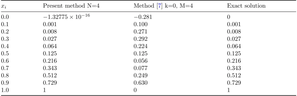
Table 3: Approximate and exact solutions for Example5.3.
xi Present method N=4 Method [7] k=0, M=4 Exact solution
0.0 −1.32775×10⁻¹⁶ −0.281 0
0.1 0.001 0.100 0.001
0.2 0.008 0.271 0.008
0.3 0.027 0.292 0.027
0.4 0.064 0.224 0.064
0.5 0.125 0.125 0.125
0.6 0.216 0.056 0.216
0.7 0.343 0.077 0.343
0.8 0.512 0.249 0.512
0.9 0.729 0.630 0.729
1.0 1 0 1
eN(x) =yα(x)−yN(x) (4.32)
Equation(4.30), give the following estimates
∥eN∥L2w(−1,1)≤C1N− 1
2−α, (4.33)
∥eN∥L∞(−1,1)≤C2N−α, (4.34)
∥eN∥Hw1(−1,1)≤C3N 1
2−α. (4.35)
whereC1, C2 and C3 are positive constants in-dependent of N. The continuous L2w(−1,1) and
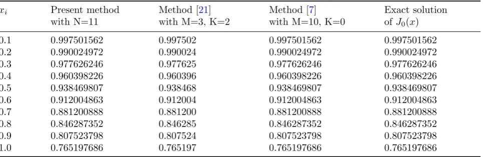
Table 4: Approximate and exact solutions for Example5.4.
xi Present method Method [21] Method [7] Exact solution
with N=11 with M=3, K=2 with M=10, K=0 ofJ0(x)
0.1 0.997501562 0.997502 0.997501562 0.997501562 0.2 0.990024972 0.990024 0.990024972 0.990024972 0.3 0.977626246 0.977625 0.977626246 0.977626246 0.4 0.960398226 0.960396 0.960398226 0.960398226 0.5 0.938469807 0.938468 0.938469807 0.938469807 0.6 0.912004863 0.912004 0.912004863 0.912004863 0.7 0.881200888 0.881200 0.881200888 0.881200888 0.8 0.846287352 0.846285 0.846287352 0.846287352 0.9 0.807523798 0.807524 0.807523798 0.807523798 1.0 0.765197686 0.765197 0.765197686 0.765197686
Table 5: Approximate and exact solutions for Example5.5.
xi Present method N=7 Method [6] N=13 Method [13] N=14 Method [9] N=20
0.0 0.828483 0.828483 0.828432 0.828483
0.1 0.829706 0.829706 0.829706 0.829706
0.2 0.833375 0.833374 0.833374 0.833374
0.3 0.839489 0.839489 0.839489 0.839473
0.4 0.848053 0.848052 0.848052 0.848052
0.5 0.859065 0.859064 0.859064 0.859064
0.6 0.872528 0.872528 0.872528 0.872528
0.7 0.888445 0.888445 0.888445 0.888445
0.8 0.906819 0.906818 0.906818 0.906818
0.9 0.927951 0.927950 0.927650 0.927650
1.0 0.950946 0.950945 0.950957 0.950945
way, the L∞(1,1)-norm is calculated by taking the maximum ofeN(x) on the aboveM+1 Gauss-Lobatto points. Numerical estimates of the order of the error, namely,eN =O(N−q).
Theorem 4.2 Suppose X = C[0,1] and
Y be Banach spaces with the norm ∥z∥=
max|z(x)|, x ∈ X. Let N : X → Y which sat-isfies the Lipschitz condition
∥y(x1)−y(x2)∥≤β∥x1−x2∥,∀x1, x2,0≤β <1. (4.36) If we assume the ∥y0∥<∞, then the sequence
sn = C + N(sn−1), converges to the exact solution y.
Proof: See [23].
Now we have to prove that the result is true for n=k+ 1.
Hence the result is true for all values of n. We complete the proof by showing that sn is a Cauchy sequence on the Banach space X.
For everym, n∈N, m≤n, we have
∥sn −sm∥= ∥(sn −sn−1) + (sn−1 −sn−2) +
. . .(sm+1−sm)∥
≤ ∥sn−sn−1∥+∥sn−1−sn−2∥+. . .+∥sm+1−
sm∥
≤ βn−1∥y0∥+βn−2∥y0∥+. . . +
βm−+1∥y0∥+βm∥y0∥
≤ ∥y0∥βm(1 +β+β2+. . .+βn−1−m) ≤ ∥y0∥βm(1−β
n−m
1−β ).
since 0< β <1, 1−βn−m<1 and ∥y0∥<∞,
∥sn−sm∥≤ ∥y0∥
βm
1−β. (4.37)
Taking limit asn, m→ ∞,
lim
n,m→∞∥sn−sm∥= 0. (4.38)
Therefore, sn is a Cauchy sequence in the Ba-nach space X. This implies that the series solu-tion ym(x) =
∑N
j=0cjTL,j(x) = CTϕ(x) by the present method is convergent to exact solutiony
5
Numerical examples
To illustrate the effectiveness of the proposed methods in the present paper, several test exam-ples are carried out in this section.
Example 5.1 Consider this problem that is co-incided by heat conduction model of the human head,
y′′(x) + 2
xy
′(x) =−e−y. (5.39)
we consider the solution this problem with condi-tion as follows:
y′(0) = 0, y(1) +y′(1) = 0. (5.40)
In this example, we do not have exact solution. We solved this equation by presented method and compared our results by method of [12, 17, 20]. The results can be seen in Table 1.
Example 5.2 Consider the singular boundary value problem for 0≤x≤1 as:
y′′(x)+0.5
x y
′(x) =ey(x)(0.5−ey(x)), (5.41)
y(0) = ln(2), y(1) = 0. (5.42)
which has the exact solutiony(x) = ln(x22+1). We
applying the method with N = 10, N = 13 and
compared the results by Wavelet method results on paper [7]. The numerical results can be seen in Table 2.
Example 5.3 Consider the singular boundary value problem, which has been considered in [7] for x∈(0,1] as:
y′′(x)+ex1y′(x)+y(x) = 6x+x3+3x2e 1
x, (5.43)
y(0) = 0, y(1) = 1. (5.44)
The exact solution of this problem is
y(x) =x3. (5.45)
We solve this problem by applying the presented method withN = 4 and compared the results by results of method [7] in Table3. As its clear from the table present method has exact solutions by small number of basis and has very better results than previous method.
Example 5.4 Consider the Bessel differential equation of order zero [21, 7]
xy′′(x) +y′(x) +xy(x) = 0, x∈(0,1] (5.46)
y(0) = 1, y′(0) = 0. (5.47)
A solution known as the Bessel function of the first kind of order of zero denoted by J0(x) is
J0(x) =
∞
∑
q=0 (−1)q
(q! )2 (
x
2)
2q. (5.48)
Table 4 compares the y(x) obtained by the pro-posed method in this paper and the method of [21] and [7].
Example 5.5 Consider the following oxygen dif-fusion problem
y′′(x) + 2
xy
′(x) = 0.76129y
y+ 0.03119, (5.49)
y′(0) = 0, 5y(1) +y′(1) = 5. (5.50)
As this problem is a real world problem we don’t have its exact answer, because of this we com-pare different numerical method answers for this example [6,13,9] that are presented in Table5.
6
Conclusion
In this paper, we implemented an efficient numer-ical method for solving the singular nonlinear dif-ferential equations. The properties of the Cheby-shev polynomials matrix of derivative are used to reduce the differential equations to a system of algebraic equations. The convergence analysis of the proposed method is introduced. From illus-trative examples, it can be seen that the proposed numerical approach can obtain very accurate and satisfactory results and has better results analogy to other existed methods.
References
[2] C. Canuto, M. Y. Hussaini, A. Quarteroni, T. A. Zang, Spectral Methods in Fluid Dy-namic,Englewood Cliffs, N. J. Prentice-Hall, 1988.
[3] A. Deb, A. Dasgupta, G. Sarkar, A new set of orthogonal functions and its applications to the analysis of dynamic cystems,J. Frank. Inst.343 (2006) 1- 26.
[4] E. H. Doha , A. H. Bhrawy, S. S. Ezz-Eldien, A Chebyshev spectral method based on operational matrix for initial and bound-ary value problems of fractional order, Com-puters & Mathematics with Applications 62 (2011) 2364-2373.
[5] T. Geyikli, S. G. Karakoc, Petrov-Galerkin method with cubic B-splines for solving the MEW equation, B. Belg. Math. Soc-Sim. 9 (2012) 215-227.
[6] E. Hashemizadeh, F. Mahmoodi, A Numer-ical Approach for the Solution of Nonlinear Boundary Value Problems Arising in Biol-ogy Via Shifted Jacobi Operational Matrix,
Advances in Environmental Biology 5 (2014) 1415-1419.
[7] A. Kazemi Nasab, A.Kilican, E. Babolian, Z. Pashazadeh Atabakan, Wavelet analy-sis method for solving linear and nonlinear singular boundary value problems, Applied
Mathematical Modelling 37 (2013)
5876-5886.
[8] Y. Khan, H. Vazquez-Leal, N. Faraz, An auxiliary parameter method using Adomian polynomials and Laplace transformation for nonlinear differential equations,Appl. Math. Model.37 (2013) 2702 - 2708.
[9] S. A. Khuri, A. Sayfy, A novel approach for the solution of a class of singular bound-ary value problems arising in physiology, J. Math. Comput. Model.52 (2010) 626-636.
[10] A. Lastra, S. Malek, J.Sanz, On Gevrey so-lutions of threefold singular nonlinear partial differential equations,Journal of Differential Equations 15 (2013) 3205-3232.
[11] Y. Liu, Piecewise continuous solutions of ini-tial value problems of singular fractional dif-ferential equations with impulse effects,Acta Mathematica Scientia 5 (2016) 1492-1508.
[12] K. Maleknejad, E. Hashemizadeh, Numeri-cal solution of nonlinear singular ordinary differential equations arising in biology via operational matrix of shifted Legendre poly-nomials, American Journal of Computa-tional and Applied Mathematics 1 (2011) 15-19.
[13] K. Maleknejad, E. Hashemizadeh, M. Mohsenyzadeh, Bernestein operational ma-trix method for solving physiology problems,
Proceeding of the international conference of Bioinformatics and Computational Biology
(2012) 276-279.
[14] F. Mirzaee, E. Hadadiyan, S. Bimesl Numer-ical solution for three-dimensional nonlinear mixed Volterra-Fredholm integral equations via three-dimensional block-pulse functions,
Appl. Math. Comput.237 (2014) 168-175.
[15] M. Nosrati Sahlan, E. Hashemizadeh, Wavelet Galerkin method for solving nonlin-ear singular boundary value problems aris-ing in physiology, Applied Mathematics and Computation 250 (2015) 260-269.
[16] K. B. Oldham, J. Spanier, The Fractional Calculus,Academic Press, New York, 1974.
[17] R. K. Pandey, Arvind K. Singh, On the con-vergence of a finite difference method for a class of singular boundary value prob-lems arising in physiology,J. Comput. Appl. Math.166 (2004) 553-564.
[18] I. Podlubny, Fractional Differential Equa-tions,Academic Press, New York, 1999.
[19] V. Prusa, K. R. Rajagopal, On the response of physical systems governed by non-linear ordinary differential equations to step
in-put, International Journal of Non-Linear
Mechanics 81 (2016) 207 - 221.
[20] J. Rashidinia, R. Mohammadi, R. Jalilian, The numerical solution of non-linear singu-lar boundary value problems arising in phys-iology, J. Appl. Math. Comput. 185 (2007) 360-367.
[22] T. Roshan, A Petrov–Galerkin method for solving the generalized regularized long wave (GRLW) equation,Comput. Math. Applic.5 (2012) 943-956.
[23] P. Roul, U. Warbbe, New approach for solving a class of singular boundary value problem arrising in various physicaly mod-els, Journal of Mathematical Chemistry 54 (2016) 1255-1285.
[24] S. Seyed Allaei, T. Diogo, M. Rebelo, An-alytical and computational methods for a class of nonlinear singular integral equations,
Applied Numerical Mathematics 114 (2017)
2-17.
[25] X. Shang, Y. Yuan, Homotopy perturbation method based on Green function for solv-ing non-linear ssolv-ingular boundary value prob-lems, International Conference on Machine Learning and Cybernetics10 (2011) 851-855.
[26] M. A. Snyder, Chebyshev Methods in Nu-merical Approximation, Prentice-Hall, Inc. Englewood Cliffs, N. J.1966.
Elham Hashemizadeh obtained her Ph.D. degree in Applied Mathe-matics in Numerical Analysis area in year 2012. She was top stu-dent in school and university. She ranked number one in M.Sc. and Ph.D. course in Islamic Azad Uni-versity Karaj Branch, also she selected as top re-searcher several times. She is now Associate Pro-fessor in Islamic Azad University Karaj Branch. Her research interests include Applied mathemat-ics, Integral Equations, Mathematics program-ming, Mathematica, Numerical Methods, Numer-ical Algorithms, Differential equations and etc.